On the Use of Regulator Theory in Neuroscience with Implications for

Robotics

Mireille E. Broucke

Electrical and Computer Engineering, University of Toronto, Toronto, Canada

Keywords:

Regulator Theory, Adaptive Internal Models, Motor Control, Cerebellum.

Abstract:

We survey recent results on the use of regulator theory in neuroscience, particularly to model the contribution

of the cerebellum to motor systems. Based on our study of the slow eye movement systems as well as visuomo-

tor adaptation, several themes emerge, including a promising structural model of the cerebellum, and insights

on how the cerebellum may enable and disable internal models. Implications for robotics are discussed at the

end of the paper.

1 INTRODUCTION

This paper presents an overview of our recent work

on applying regulator theory to problems of neuro-

science, particularly modeling the contribution of the

cerebellum to human motor systems. We present

a structural model that is inspired by the cerebellar

anatomy. This model will be recognizable as an adap-

tive observer. Our working hypothesis is that the pri-

mary function of the cerebellum is disturbance rejec-

tion of exogenous reference and disturbance signals.

This interpretation of cerebellar function places the

internal model principle at front and center (Francis

and Wonham, 1976). The idea to interpret the cere-

bellum in terms of disturbance rejection is not new.

For instance, the ﬁrst proposal by Stephen Lisberger

on the role of internal models in the cerebellum in

his survey paper (Lisberger, 2009) is consistent with

a role of disturbance rejection. Lisberger describes

internal models as providing “a model of the inertia

of real-world objects in motion”; see also (Cerminara

et al., 2009). What is new is our use of regulator the-

ory to mathematically model the cerebellum.

This paper is informal. We suppress mathematical

details as much as we can, without necessarily com-

promising on completeness. We want to draw con-

nections between different areas that are typically not

compared side by side: for instance, regulator designs

for disturbance rejection with a systems-level model

of the cerebellum; speciﬁc models of motor systems

compared with each other; even comparisons between

continuous-time and discrete-time processes both as-

sociated with the cerebellum. In making this sur-

vey, several themes or takeaways emerge, which we

already summarize here for the reader who is inter-

ested in the main points (meanings of speciﬁc terms

are found in the main text below):

• The cerebellar architecture resembles that of an

adaptive observer (Kreisselmeier, 1977; Kanel-

lakopoulos and Kokotovic, 1995).

• The nucleo-cortical pathway is in direct corre-

spondence with the internal model principle in

the sense that without this pathway, the inter-

nal model principle would not be satisﬁed by the

mathematical model.

• The theory suggests that the granular layer ﬁlters

of the cerebellum must synchronize on the same

time constants for ﬁltering mossy ﬁber (MF) in-

puts to the same cerebellar modules.

• Mathematically speaking, there is considerable

ﬂexibility in terms of how MF inputs to the cere-

bellum may be combined or “pre-bundled”.

• The mathematical models suggest that some MF

inputs have the role to ensure that they are not

cancelled out by the cerebellum. This seemingly

contradictory role may potentially lead to misin-

terpretations of the function of certain cerebellar

modules. On the other hand, the collaborative role

between the cerebellum and feedforward signals

is well known.

• The cerebellum may well be the unique brain

structure that is wired to handle the dangerous op-

eration of shutting on and off internal models for

satisfaction of the internal model principle.

• Research on the cerebellum has implications for

robotics.

Broucke, M.

On the Use of Regulator Theory in Neuroscience with Implications for Robotics.

DOI: 10.5220/0010639100110023

In Proceedings of the 18th International Conference on Informatics in Control, Automation and Robotics (ICINCO 2021), pages 11-23

ISBN: 978-989-758-522-7

2 CEREBELLUM

The locus of internal models in the brain is believed to

be the cerebellum. The cerebellum is a major brain re-

gion positioned at the back of the head, partly covered

by the cerebral cortex, and itself covering the brain-

stem. In 1967 nobel prize winner John Eccles and

his co-authors laid out the microcircuit of the cerebel-

lum (Eccles et al., 1967). Their work showed that the

cerebellum contains relatively few neuron types, and

that it has a laminated structure with a repeating ar-

chitectural pattern pervading each layer or functional

module. Each module has only two input pathways

and a single output pathway (Apps et al., 2018).

The ﬁrst of two input pathways to the cerebellum

is via the mossy ﬁber (MF) inputs. The MFs carry a

rich ﬂow of information from sensory inputs as well

as the output of the cerebellum itself. Mossy ﬁber out-

puts are received by tens of billions of granule cells,

the most common cell type of the brain. The axons

of the granule cells form parallel ﬁbers, which con-

nect with the dendrites of the principal neuron type of

the cerebellum, the Purkinje cells (PCs). Each PC re-

ceives synaptic connections from as many as 200,000

parallel ﬁbers, resulting in a massive fan-in of infor-

mation. The second input pathway to the cerebellum

is via the climbing ﬁbers, which are the axons of cells

from part of the brainstem called the inferior olive.

The climbing ﬁber input carries a sensory error signal,

and each climbing ﬁber forms a powerful connection

with a single PC. Climbing ﬁbers are capable to mod-

ify the strength of the synapse between parallel ﬁber

inputs onto the PCs. The PC axons project to the deep

cerebellar nuclei and the vestibular nuclei, forming

the only output pathway from the cerebellum.

Notable features of the anatomical structure from

a control perspective are:

(i) The cerebellum has a purely feedforward struc-

ture. Information ﬂows from the MF inputs to

granule cells and then via the parallel ﬁbers to

the PCs. The PCs send their outputs to the deep

cerebellar nuclei and vestibular nuclei.

(ii) Each functional module of the cerebellum is

identical to the others and performs the same

neural computation. The only distinction be-

tween modules is in terms of the input and output

connections to other regions of the brain.

(iii) Each functional module of the cerebellum pro-

cesses its own sensory error signal received via

the climbing ﬁber inputs from a circumscribed

region of the inferior olive. Each module sends

its output to a circumscribed region in the cere-

bellar nuclei or vestibular nuclei.

(iv) The adaptive capability of the cerebellum is pro-

vided by the climbing ﬁber input which changes

the strength of the synapse between the parallel

ﬁbers and the PCs.

(v) Mossy ﬁbers projecting to a similar region of the

cerebellar cortex encode similar information.

(vi) Each of the deep cerebellar nuclei and the

vestibular nuclei has a projection to the MF in-

puts of the cerebellum. This projection is termed

the nucleo-cortical pathway and is regarded to

provide an efference copy of the motor command

issued by the cerebellum (Ruigrok, 2011; Houck

and Person, 2014).

3 STRUCTURAL MODEL

The features we have highlighted suggest a struc-

tural model associated with a single cerebellar mod-

ule. This model that does not reveal function but ac-

cords with cerebellar structure at a systems level:

˙x = Ax + Bu + Ed

(3.1a)

e = Cx + Dd

(3.1b)

˙w

= F

+ G

m f ,1

(3.1c)

˙w

= F

+ G

m f ,k

(3.1d)

˙w

k+1

= F

k+1

+ G

k+1

(3.1e)

ˆw = (w

, . . . , w

k+1

) (3.1f)

ψ = γe ˆw

(3.1g)

ψ ˆw (3.1h)

u = u

+ u

. (3.1i)

Equation (3.1a) represents the open-loop system un-

der regulation by the cerebellum: horizontal eye po-

sition, eye velocity, hand position, hand grip force,

gait, stance, and so forth. Signal e ∈ R is an er-

ror that the cerebellum is tasked with asymptotically

driving to zero. Signal d

∈ R is a persistent exoge-

nous disturbance entering at the plant input. Signal

∈ R is a persistent exogenous disturbance entering

at the error measurement. Distinct MF input signals

are u

m f ,1

, . . . , u

m f ,k

, u

∈ R, which arrive by way of

the ﬁlters (3.1c)-(3.1e) with corresponding ﬁlter states

, . . . , w

k+1

. We assume each F

, i = 1, . . . , k + 1 is

Hurwitz. These ﬁlters are in analogy with the lead-lag

ﬁlters utilized in (Fujita, 1982) to model the granular

layer, but we allow a more general interpretation here.

The ﬁlter (3.1e) is particularly important as it mod-

els the nucleo-cortical pathway. The equation (3.1g)

is the standard least-mean-squares (LMS) parameter

adaptation law to model the modiﬁable synapses be-

tween parallel ﬁbers and PCs. The signal e in (3.1g) is

ICINCO 2021 - 18th International Conference on Informatics in Control, Automation and Robotics

supplied by the climbing ﬁber input. Parameter γ > 0

is the adaptation rate. The output of the cerebellum is

, and the motor command is u, which includes u

for closed-loop stability, if needed. A control theorist

will recognize the structural model to be an adaptive

observer (Kreisselmeier, 1977; Kanellakopoulos and

Kokotovic, 1995).

4 DISTURBANCE REJECTION

The structural model does not endow the cerebellum

with any particular function except that of ﬁltering

MF inputs with parameter adaptation. Our working

hypothesis is that the primary function of the cerebel-

lum is disturbance rejection, bringing into view regu-

lator theory (Wonham, 1985). In this section we look

at a representative regulator design to solve the dis-

turbance rejection problem so that we can bring out

comparisons with the structural model. The design

utilizes adaptive internal models (Nikiforov, 2004a;

Nikiforov, 2004b).

Consider the open-loop system

˙x = Ax + B(u + d) (4.1a)

˙w = Fw + Gd (4.1b)

d = ψw (4.1c)

e = Cx , (4.1d)

where x ∈ R

is the state, w ∈ R

is the exosystem

state, u ∈ R is the control input, e ∈ R is the error

to be regulated, and d ∈ R is a persistent, exogenous

disturbance signal entering the plant at the control in-

put. The exosystem (4.1b) provides a model of the

frequency content of the disturbance in terms of a row

vector of unknown parameters ψ ∈ R

1×q

Problem 4.1 (Regulator Problem). Consider the sys-

tem (4.1). Find a error feedback regulator

˙x

= Fx

+ Ge (4.2a)

u = Hx

+ Ke , (4.2b)

with regulator state x

(t) ∈ R

, such that the follow-

ing conditions are met:

(AS) The equilibrium (0, 0) ∈ R

× R

of the unforced

closed-loop system

˙x = (A + BKC)x + BHx

(4.3a)

˙x

= Fx

+ GCx (4.3b)

is asymptotically stable.

(R) The forced closed-loop system satisﬁes: for

all initial conditions (x(0), x

(0), w(0)), e(t) −→

0. /

The following assumptions are standard in the

regulator theory literature; see (Saberi et al., 2000)

for more background: (A1) (A, B) is controllable.

(A2) (C, A) is observable. (A3) S := F + Gψ has

simple eigenvalues on the imaginary axis. (A4)

det



A − λI B

C 0



6= 0 for all λ ∈ σ(S). (A5) (F, G) is

controllable, F is Hurwitz, and (ψ, S) is w.l.o.g. an

observable pair. (A6) An upper bound on q is known,

but the parameters of (ψ, S) are unknown. (A7) The

parameters (A, B,C) are known. (A8) The measure-

ment is x.

Consider a control input of the form (3.1i). The

ﬁrst component u

is selected for stabilization: choose

= Kx such that (A + BK) is Hurwitz. The sec-

ond component u

is designed to satisfy the inter-

nal model principle (Francis and Wonham, 1976).

Consider an adaptive internal model from (Nikiforov,

2004a):

˙w

= Fw

+ FNx (4.4a)

˙w

= Fw

− NAx (4.4b)

˙w

= Fw

− NBu (4.4c)

ˆw = w

+ Nx + w

+ w

(4.4d)

ψ = γ(B

Px) ˆw

(4.4e)

= −

ψ ˆw, (4.4f)

where N satisﬁes NB = G,

ψ is an estimate of ψ, γ > 0

is the adaptation rate, and P ∈ R

n×n

is the symmet-

ric, positive deﬁnite solution of the Lyapunov equa-

tion (A + BK)

P + P(A + BK) = −Q, with Q ∈ R

n×n

symmetric and positive deﬁnite.

Now we observe

ˆw = Fw

+ FNx + N(Ax + Bu + Bd)

+ Fw

− NAx + Fw

− NBu

= F ˆw + Gd . (4.5)

Thus, ˆw evolves according to the same dynamics as in

(4.1b). Deﬁne the estimation error

w = w − ˆw. Then

w = F

w, and since F is Hurwitz,

w(t) −→ 0, so ˆw pro-

vides an estimate of the exosystem state w. Further,

(4.4) satisﬁes the internal model principle by way of

(4.4c). For suppose that

ψ = ψ. Substituting u into

(4.4c), we have

˙w

= Fw

− NB(u

+ u

)

= (F + Gψ)w

+ Gη

where η

= ψ(w

+Nx + w

)− u

. As such, this ﬁlter

includes the unstable poles of the exosystem. Finally,

the following result is proved in (Battle and Broucke,

2021).

Theorem 4.1. Consider the system (4.1) satisfying

Assumptions (A1)-(A8), and the regulator (4.4). Sup-

pose A + BK is Hurwitz. Then this regulator solves

the disturbance rejection problem.

On the Use of Regulator Theory in Neuroscience with Implications for Robotics

In comparing (4.4) with (3.1), there are three im-

portant points:

(i) The ﬁlter (4.4c), which fulﬁlls the requirements

of the internal model principle, corresponds to the

nucleo-cortical pathway in (3.1e).

(ii) The model (4.4) bundles together ﬁlter inputs Nx,

Ax, and Bu in (4.4a)-(4.4c) based on prior knowl-

edge of the plant parameters. However, these ﬁlter

inputs need not be aggregated in this way. Mathe-

matically speaking, states or other sensory inputs

may arrive as ﬁlter inputs according to a number

of patterns or combinations, potentially depend-

ing on the structure of the open-loop system. This

mathematical ﬂexibility, in turn, may imply that

an “unpacking” of MF inputs to the cerebellum is

necessary to determine their constituent compo-

nents, making the modeling problem more chal-

lenging.

(iii) The model (4.4) requires that all the ﬁlters (4.4a)-

(4.4c) have synchronized to utilize the same ﬁl-

ter time constants, i.e. F

= F

. Since the ﬁl-

ters (3.1c)-(3.1e) or (4.4a)-(4.4c) are nominally

intended to model the granular layer of the cere-

bellum, this raises the question of whether the

granular layer is capable of some form of dynamic

synchronization.

While we have identiﬁed intriquing analogies be-

tween cerebellar structure and internal model designs

for disturbance rejection from regulator theory, the

comparison is still somewhat superﬁcial. The ocu-

lomotor system, discussed in the next section, pro-

vides more concrete evidence that such analogies can

be fruitful toward model building.

5 OCULOMOTOR SYSTEM

The oculomotor system comprises several eye move-

ment systems: the vestibulo-ocular reﬂex (VOR), op-

tokinetic system (OKS), the gaze ﬁxation system, the

smooth pursuit system, the vergence system, and the

saccadic system. The oculomotor system provides a

good starting point for studying the cerebellum be-

cause it has a very simple plant (the eyeball), and it

is believed to provide the blueprint for all other motor

systems (Leigh and Zee, 2015).

5.1 VOR, Smooth Pursuit, and Gaze

Holding

In (Broucke, 2020; Broucke, 2021) we presented a

model of the VOR, smooth pursuit, and gaze holding

r − x

−

FTN

˙x

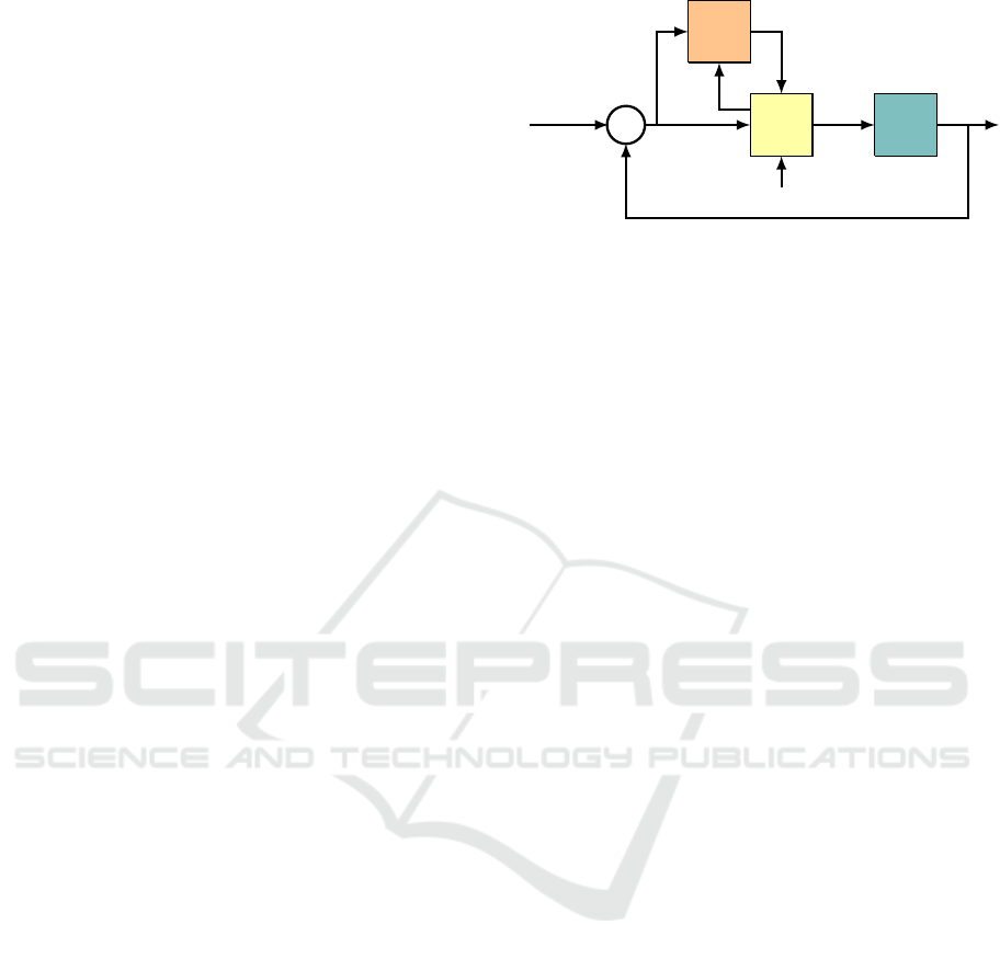
Figure 1: Control architecture for the VOR, gazing holding,

and smooth pursuit systems.

for horizontal motion of one eye by applying an adap-

tive internal model design from (Serrani and Isidori,

2000; Serrani et al., 2001). Let x ∈ R be the horizon-

tal eye angle, x

the horizontal head angle, and r the

horizontal angular position of a target. The model is:

˙x = −K

x + u (5.1a)

e = r − x − x

(5.1b)

ˆx = −K

ˆx + u (5.1c)

˙w

= Fw

+ Gu

(5.1d)

˙w

= Fw

+ Gu

(5.1e)

ˆw := w

+ w

(5.1f)

ψ = γe ˆw

(5.1g)

= α

ˆx − α

VOR

˙x

(5.1h)

= K

e (5.1i)

ψ ˆw (5.1j)

u = u

+ u

. (5.1k)

Equation (5.1a) is the ﬁrst order model of the oculo-

motor plant (Sylvestre and Cullen, 1999). Equation

(5.1b) is the retinal error, the difference between the

target angle r and the gaze angle x + x

. It is this er-

ror that the cerebellum is tasked with driving asymp-

totically to zero. Equation (5.1c) models the brain-

stem neural integrator (Robinson, 1974) which acts

as an observer to provide an estimate ˆx of eye position.

Equations (5.1d)-(5.1g) comprise the adaptive inter-

nal model in the cerebellum. The motor command

u has a component u

corresponding to a brainstem-

only pathway for pure feedforward signals, a compo-

nent u

= K

e to improve closed-loop stability, and

, the cerebellar output from the PCs.

The model can be compared to the known neural

circuit associated with these eye movement systems

uttner and B

uttner-Ennever, 2006), visualized by a

block diagram in Figure 1. The error signal (5.1b)

is transmitted from the visual cortex to the inferior

olive (IO), where it is relayed to appropriate climbing

ﬁber inputs (CFs) of the cerebellum (C), speciﬁcally,

the module called the ﬂoccular complex. This is the

signal e appearing in (5.1g). The cerebellum also re-

ICINCO 2021 - 18th International Conference on Informatics in Control, Automation and Robotics

ceives MF inputs from the medial vestibular nuclei

(MVN) in the brainstem (B). These are the MF inputs

in (5.1d)-(5.1d). The sole output of the cerebellum is

, transmitted via its PCs to ﬂoccular target neurons

(FTNs) in the MVN (Ramanchandran and Lisberger,

2008). The MVN also receives a head velocity sig-

nal from the semicircular canals of the ear, signal ˙x

in (5.1h), corresponding to the VOR. The parameter

VOR

is the VOR gain. The eye position signal α

ˆx

corresponds to the projection from the brainstem nu-

cleus prepositus hypoglossi (NPH) to the MNs. The

output of the MVN is sent both to the neural integra-

tor (NI) in the NPH and directly to the oculomotor

neurons (MNs) of the oculomotor plant (P).

As we discussed above, the MF inputs in (5.1d)-

(5.1e) may be bundled in a number of ways with no

effect on the overall behavior. For example, the two

ﬁlters could be combined into one, as was done in

(Serrani and Isidori, 2000), for a more parsimonious

model

ˆw = F ˆw + G(u

+ u

This modiﬁcation affects the choice of parameters be-

ing adapted, but it does not affect overall model be-

havior. Alternatively one could write

˙w

= Fw

+ FGe

˙w

= Fw

+ G(u − u

)

ˆw := (w

, w

)

The feedforward signals in u

are now arriving as MF

inputs to be subtracted from the overall motor com-

mand. This subtraction of feedforward signals is re-

quired so that their effect is not cancelled by the cere-

bellum (the cerebellum provides a top-up to the ac-

tion of feedforward signals). Depending on the origin

of the constituent components of the motor command

u in the brain, such an explicit subtraction of certain

MF inputs may arise, if not for the ﬂoccular complex,

possibly in another cerebellar module. Such a situ-

ation would certainly cloud an understanding of the

role of certain MF inputs to the cerebellum.

The model (5.1) recovers the standard lesion,

behavioral, and neurological experiments associated

with the VOR, gaze holding, and smooth pursuit; see

(Broucke, 2020; Broucke, 2021). Here we discuss

two interesting experiments which highlight the spe-

cial capabilities of the cerebellum.

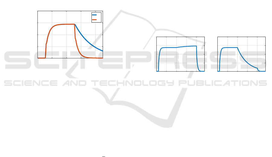
A ﬁrst experiment called the error clamp explores

the role of the error signal using a technique called

retinal stabilization (Barnes et al., 1995; Morris and

Lisberger, 1987; Stone and Lisberger, 1990). A mon-

key is trained to track a visual target moving hor-

izontally at constant speed. After reaching steady-

state, the error is optically clamped at zero using an

experimental apparatus that centers the target image

directly on the fovea. In experiments it is observed

that, despite zero error, the eye continues to track the

target for some time after. Neuroscientists postulate

so called extraretinal signals drive the smooth pur-

suit system. Figure 2 depicts the error clamp with

our model, showing on the left that the eye contin-

ues to track the target despite the measurement being

clamped at e ≡ 0 during the time interval t ∈ [5, 6].

The right ﬁgure shows the (physical) error, showing

that tracking is not robust during the time interval that

the measurement is clamped. In the second exper-

iment called target blanking, a horizontally moving

target is temporarily occluded, yet the eye continues

to track the target (Cerminara et al., 2009; Churchland

et al., 2003); researchers have postulated the brain has

an internal model of the motion of the target. In-

deed, direct measurement of the appropriate PCs of

the cerebellum shows that they remain active during

the time that the target is occluded.

0 2 4 6 8 10

Time (secs)

Eye Angle (deg)

0 2 4 6 8 10

Time (secs)

-0.4

-0.2

0.2

0.4

0.6

0.8

Error

Figure 2: Smooth pursuit with an error clamp during t ∈

[5, 6]s. The eye angle x on the left and the error e on the

right.

Let’s consider the meaning of these experiments

in terms of (5.1). In the ﬁrst experiment, the error is

clamped at zero, so we can set e ≡ 0 to obtain

˙w

= Fw

˙w

= Fw

+ Gu

ˆw := w

+ w

Since F is Hurwitz, the ﬁrst ﬁlter state w

in steady-

state is zero. Then the second ﬁlter evolves according

to ˙w

= (F + Gψ)w

, where F + Gψ is marginally

stable by (A3) (and assuming parameters have con-

verged). Clearly w

provides the drive for continued

pursuit during the error clamp, and it depends on the

nucleo-cortical pathway. However, in the second ex-

periment there is no error signal while the target is

occluded. It would certainly be paradoxical for the

cerebellum to continue to supply (on its own) a drive

for pursuit when there is no sensory error. We pos-

tulate that a higher brain center gates the activity of

the nucleo-cortical pathway. When there is no error

signal and/or the subject is not interested in an exter-

nal stimulus, then the pathway is disabled in order to

On the Use of Regulator Theory in Neuroscience with Implications for Robotics

arrive at the stable model

˙w

= Fw

˙w

= Fw

ˆw := w

+ w

, ,

in which all ﬁlter states gradually decay to a quies-

cent level of activity. However, when the error signal

is temporarily dropped but the subject remains inter-

ested in the stimulus (e.g. a lion pursuing prey), then

the nucleo-cortical pathway is not disabled. Finally,

these experiments raise intriguing questions for reg-

ulator theory. Are there engineering contexts when

a regulator should be capable to distinguish no error

measurement from a zero error measurement?

5.2 Optokinetic System

In the previous section we considered a model of a

part of the cerebellum, the ﬂoccular complex (FC),

involved in regulation of the vestibulo-ocular reﬂex,

smooth pursuit, and gazing hold eye movement sys-

tems. This section discusses a second functional mod-

ule of the cerebellum, the nodulus-uvula (NU) which

is responsible for regulating the optokinetic system.

The optokinetic system is an eye movement sys-

tem to stabilize vision on a full-ﬁeld moving visual

surround. This eye movement system contrasts with

the eye movement systems of the previous section

whose goal is to stabilize an object on the fovea. How

the optokinetic system interacts with the other eye

movement systems is of great interest scientiﬁcally,

but also theoretically from the perspective of control

theory: can parallel adaptive internal models work

collaboratively to regulate the same error? Or does the

brain utilize a switching mechanism to switch from

one adaptive internal model to the other, reminiscent

of switched system architectures for adaptive control

(Narendra and Annaswamy, 1989)?

Pioneering experimental work in the 1970’s on the

optokinetic system (Cohen et al., 1977; Raphan et al.,

1979; Waespe and Henn, 1978a; Waespe and Henn,

1978b) lead to the discovery of the velocity storage

mechanism (VSM), a behavior in which eye velocity

is stored while following a constant velocity visual

surround, even with intervening saccades (a fast reset

of eye position) in a behavior called nystagmus. A

striking feature of the VSM is that it partially meets

the requirements of the internal model principle, as if

evolution made a ﬁrst attempt at architecting a neural

internal model.

In (Battle and Broucke, 2021) we proposed a

model of the optokinetic system given by

˙x

= x

(5.2a)

˙x

= α

(−x

− K

+ u) (5.2b)

e = ˙x

− ˙x

− x

(5.2c)

ˆx = −K

ˆx + u (5.2d)

˙v = −K

v + K

e (5.2e)

˙w

= Fw

+ FGe (5.2f)

˙w

= Fw

− Ge (5.2g)

˙w

= Fw

− Gu

(5.2h)

˙w

= Fw

− G ˆx (5.2i)

˙w

= Fw

− G ˙x

(5.2j)

˙w

= Fw

− Gv (5.2k)

ˆw = (w

+ Ge, w

, w

) (5.2l)

ψ = γe ˆw

(5.2m)

ψ ˆw (5.2n)

= α

ˆx − α

VOR

˙x

+ α

e + α

v (5.2o)

u = u

+ u

. (5.2p)

We utilized a second-order model of the oculomo-

tor plant in (5.2a)-(5.2b), with x

the horizontal eye

angle and x

the eye angular velocity, because the op-

tokinetic system stabilizes eye velocity, not eye posi-

tion. The error signal e in (5.2c) to be regulated by the

cerebellum is the retinal slip velocity, the difference

between the horizontal angular velocity of the visual

ﬁeld ˙x

and the gaze velocity x

+ ˙x

. A non-zero

˙x

is induced in experiments when a subject is seated

inside a rotating optical drum. The brainstem neural

integrator again appears in (5.2d). Equation (5.2e) is

the velocity storage integrator of the optokinetic sys-

tem (Cohen et al., 1977). The motor command u is

now regarded as an acceleration input; v is the state

of the velocity storage integrator; α

e captures the

drive provided by the optokinetic reﬂex, where α

the called the optokinetic gain; the vestibulo-ocular

reﬂex is modeled by α

VOR

˙x

, as before. The term α

captures the drive provided by the velocity storage in-

tegrator. Finally, we mention that there is no stabi-

lizing feedback u

in this model because the velocity

dynamics of the oculomotor plant are already highly

stable.

In comparing this model to the structural model

(3.1), we observe the additional ﬁlters (5.2f)-(5.2k)

driven by feedforward signals ˆx, ˙x

, and v. Mathe-

matically speaking, it can be shown that if these sig-

nals are not included as MF inputs, then they would

be cancelled or rejected by the activity of the nodu-

lus/uvula as predicted by the model. Thus, a pattern

we have already highlighted on the variable roles of

certain MF inputs is reinforced again with this model:

mathematically speaking, MF inputs may either ap-

ICINCO 2021 - 18th International Conference on Informatics in Control, Automation and Robotics

pear because they are directly involved in disturbance

estimation or they appear to avoid being cancelled by

the cerebellum.

The model (5.2) is consistent with the neural cir-

cuit, and it recovers ﬁve standard behaviors of the op-

tokinetic system: optokinetic nystagmus (OKN); op-

tokinetic after-nystagmus (OKAN I); OKAN suppres-

sion; OKN suppression; and OKAN II. For instance,

OKN is an eye movement in which the eye tracks the

velocity of a (full-ﬁeld) moving visual surround dur-

ing the so-called slow phase, followed by a saccade to

rapidly reset the eye position to zero in the fast phase

(Cohen et al., 1977; Raphan et al., 1979). OKAN I is

a behavior following OKN when the lights are turned

off. During OKAN I nystagmus continues in the same

direction as OKN, even though there is no visual stim-

ulation (Cohen et al., 1977; B

uttner et al., 1976).

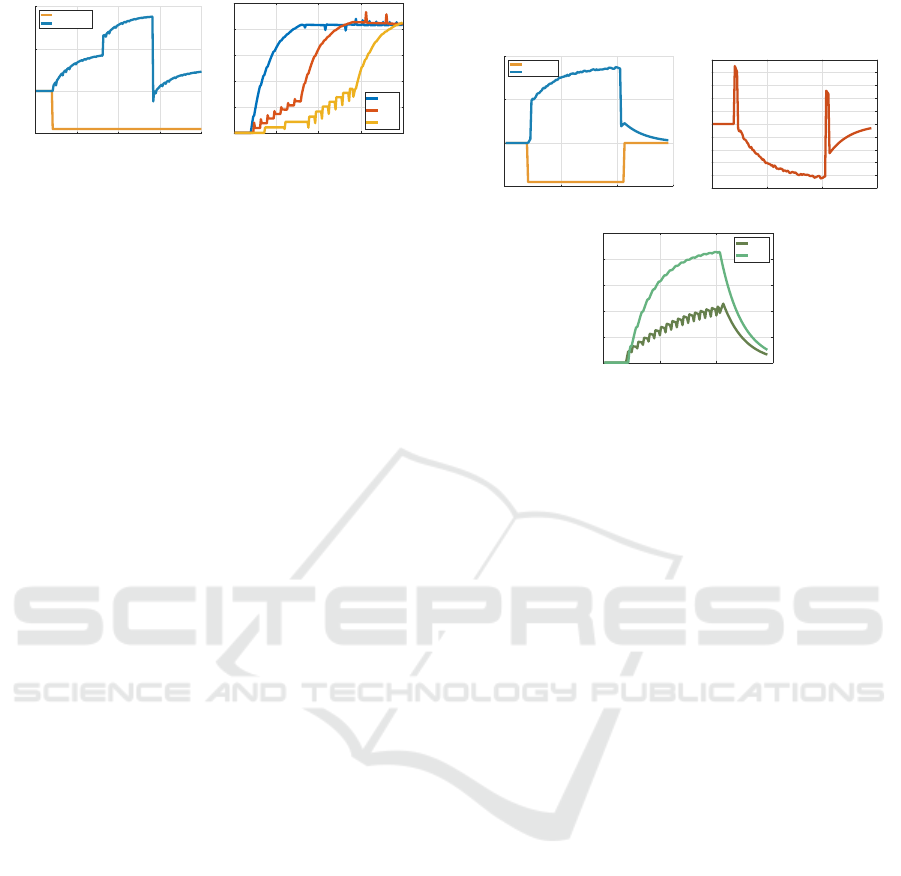
Figure 3 shows simulation results for OKN and

OKAN I using our model, with the optokinetic drum

rotating at a constant velocity of 60 deg/s for 60s. The

initial jump in slow phase eye velocity is attributable

to the large retinal slip velocity at the onset of the

experiment and the charging of the VSM. The non-

zero steady-state error during OKN is observed be-

cause the NU internal model is “untrained”. Once the

lights are extinguished at t = 60s, visual signals are no

longer present and the cerebellum is effectively inac-

tive, the signal e is unavailable, and u

= 0 (based on

gating the nucleo-cortical pathway). This causes the

slow-phase eye velocity to rely on the dynamics from

the VSM, which slowly dissipates its stored velocity,

creating OKAN I.

If the subject is involved in repeated trials of the

same experiment eliciting OKN and OKAN I, the

NU internal model is “trained” over time. Conse-

quently, the OKN steady-state slow-phase eye veloc-

ity increases (Miki et al., 2020, Fig 1); the OKAN

I time constant decreases (Cohen et al., 1977, Fig

7); and the OKAN I duration decreases (Waespe and

Henn, 1978b, Fig 2, 3). These results are shown on

the right of Figure 3.

0 50 100 150 200

Time (secs)

Stimulus and Eye Velocities (deg/s)

0 50 100 150 200

Time (secs)

Stimulus and Eye Velocities (deg/s)

Figure 3: Untrained (left) and trained (right) OKN and

OKAN I.

This section has demonstrated that a disturbance

rejection interpretation of cerebellar function can be

propitious to arrive at plausible models for one mo-

tor system: the oculomotor system. However, one

may also utilize regulator theory to understand other

adaptive behaviors that are best modeled as discrete,

repetitive processes. Perhaps the most widely studied

adaptive, discrete process is visuomotor adaptation,

considered in the next section.

6 VISUOMOTOR ADAPTATION

Visuomotor adaptation is a subconscious, “machine-

like” brain process taking place over repetitive trials

and elicited by a visual error closely following the

execution of a movement. Visuomotor adaptation is

intended to calibrate over a lifetime the mapping be-

tween what is seen and how to move. As a means

to expose the underlying computations of this brain

process, neuroscientists create experiments that ar-

tiﬁcially perturb what is seen by the subject during

movement. Examples include saccades with an inter-

saccadic step of the target (Kojima et al., 2004); the

visuomotor rotation experiment with fast arm reaches

(Smith et al., 2006; Shadmehr and Wise, 2005); and

throwing darts while looking through prism glasses

(Martin et al., 1996).

Visuomotor adaptation experiments consist of

repetitive trials of a certain movement such as a sac-

cade or arm reach. The trials are classiﬁed by type,

and sequences of blocks of trials of speciﬁc types are

utilized to elicit so-called dynamic behaviors of adap-

tation. A baseline (B) block familiarizes the subject

with the experimental aparatus under unperturbed,

normal conditions. A learning (L) block occurs after

a baseline block when a perturbation or disturbance is

introduced. A washout (W) block follows a learning

block when the perturbation is removed. An unlearn-

ing (U) block follows a learning block when the per-

turbation changes in sign but not magnitute relative to

the learning block. A relearning (R) block is a second

learning block with the same perturbation. A down-

scaling block (D) is a second learning block in which

the perturbation is set to a fraction of its value in the

ﬁrst learning block. A no-visual-feedback (N) block

is a block of trials in which no error measurement is

presented to the subject. An error clamp (C) block

is a block of trials when the error measurement pre-

sented to the subject is clamped artiﬁcially to a value

unrelated to the subject’s movements. When blocks

of trials are sequenced in a particular order and with a

particular number of trials in each block, then several

phenomena emerge in experiments:

• Savings is a behavior in which learning is sped up

in the second learning block relative to the ﬁrst

one.

On the Use of Regulator Theory in Neuroscience with Implications for Robotics

• Reduced savings is a behavior in which savings is

reduced by inserting a washout block of trials after

the unlearning block. After the washout block,

relearning does not proceed as rapidly as in the

savings experiment.

• Anterograde interference is a behavior in which

a previously learned task reduces the rate of sub-

sequent learning of a different (and usually oppo-

site) task.

• Rapid unlearning is a behavior in which the rate

of unlearning is faster than the rate of initial learn-

ing, if the number of trials in the learning block is

small.

• Rapid downscaling is a behavior in which the rate

of learning in a secondary learning block is faster

when the rotation is set to a fraction of its value in

the initial learning block.

• Spontaneous recovery is a behavior observed dur-

ing the washout block of a BLUW experiment

in which the response partially “rebounds” to its

value at the end of the learning block rather than

converging monotonically to zero.

0 100 200 300

Trial

-40

-20

Disturbance

0 100 200 300

Trial

x(k)

0 10 20 30

Trial

x(k)

Learning

Relearning

Figure 4: Savings in a BLUR experiment. In the bottom

ﬁgure x(k) during the learning block is plotted in blue su-

perimposed with a horizontally shifted version of x(k) dur-

ing the relearning block in purple. The purple curve is larger

than the blue curve corresponding to faster learning in the

relearning block.

We used regulator theory to develop a model of

visuomotor adaptation in (Gawad and Broucke, 2020;

Hafez et al., 2021) with the goal to recover the six

standard behaviors of visuomotor adaptation. The

model was based on three assumptions. First, we

focused on motor adaptation tasks involving one de-

gree of freedom of movement; for instance, horizon-

tal movement of the eye, hand angle relative to a ref-

erence angle in a horizontal plane, forward (coronal)

inclination of the body relative to a vertical reference,

the horizontal angle of a dart thrown by a subject, and

so forth. Second, we assumed the open-loop model is

linear time-invariant. Third, we focused on constant

disturbances, as currently there is a dearth of experi-

ments with non-constant disturbances.

Let integer k be the trial number; x(k) is the state

of a single degree of freedom of the body at the end

of the k-th trial; d(k) is an additive disturbance in the

measurement during the k-th trial; and e(k) is the error

between a measurement y(k) = x(k) + d(k) observed

by the subject at the end of the k-th trial and a ref-

erence r(k). Our discrete-time model of visuomotor

adaptation is:

x(k + 1) = Ax(k) + Bu(k) (6.1a)

e(k) = r(k) − d(k) − x(k) (6.1b)

(k + 1) = Fw

(k) + FGe(k) (6.1c)

(k + 1) = Fw

(k) − Ge(k) (6.1d)

(k + 1) = Fw

(k) − Gu(k) (6.1e)

ˆw(k) = (w

(k) + Ge(k), w

(k), w

(k)) (6.1f)

u(k) = Ke(k) + K

ψ ˆw(k). (6.1g)

The open-loop system model (6.1a) provides a high-

level, abstract description of the quantitative change

over successive trials of a single degree of freedom of

the body. The term Ax(k) models a retention or mem-

ory mechanism of the state in the previous trial. We

assume the ﬁlters (6.1c)-(6.1e) are stable; that is, F is

Schur stable. We have not written a parameter adap-

tation law for unknown parameters ψ (although one

may do so) since experiments show that the parame-

ters vary extremely slowly; see (Gawad and Broucke,

2020). The controller u has the same components

as before: u

(k) = Ke(k) is to improve closed-loop

stability, while u

= K

ψ ˆw(k) is the component to

satisfy the internal model principle. The parameter

0 < K

< 1 is explained below.

Figures 4 shows a simulation for a BLUR exper-

iment to elicit savings. The top left ﬁgure shows the

disturbance value d(k) as a function of k, and the top

right ﬁgure shows x(k). The bottom ﬁgure shows x(k)

during the learning block superimposed with x(k) dur-

ing the relearning block. We see that relearning is

faster than learning, demonstrating that savings have

indeed occurred in the relearning block.

Visuomotor adaptation experiments analogous to

the error clamp and target blanking experiments for

the smooth pursuit system have also been performed.

These provide dramatic evidence of the brain’s capa-

bility to enable or disable internal models. For in-

stance, many experimental studies of the form BLN

have been conducted on the effect of removing the vi-

sual error in an N block following a learning block

(Galea et al., 2011; Kitago et al., 2013; Bond and

Taylor, 2015). The major ﬁnding is that during the N

block, x(k) slowly returns to a nominal reference po-

ICINCO 2021 - 18th International Conference on Informatics in Control, Automation and Robotics

sition. Further, Figure 2 of (Kitago et al., 2013) shows

that the rate of decay is faster in a W block than an N

block.

As we already discussed for the oculomotor sys-

tem, when there is no error measurement, we must

remove the signal e(k) from every ﬁlter input in (6.1).

To disable the internal model, it is also necessary to

disable the efference copy u(k) in (6.1e). The re-

sulting internal model will consist of ﬁlters that are

all stable, and therefore the response x(k) will grad-

ually return to a zero reference value. In summary,

if we assume that visuomotor adaptation operates in

a manner that is consistent with the oculomotor sys-

tem, then gating the nucleo-cortical pathway provides

an explanation for how internal models can be en-

abled or disabled in visuomotor adaptation. Figure 5

shows the results for (6.1) for a BLN experiment us-

ing this method to disable the internal model during

the N block.

0 20 40 60 80

Trial

x(k)

Figure 5: BLN experiment v.s. BLW experiment.

A number of error clamp experiments of the form

BLC(µ) have been reported including (Smith et al.,

2006; Kitago et al., 2013; Shmuelof et al., 2012;

Vaswani et al., 2015). In these experiments a sub-

ject makes fast arm reaches to a target on a computer

screen while observing a cursor intended to represent

the hand position at the end of a reach. A disturbance

d(k) is introduced during the learning blocks so that

the observed cursor angle is y(k) = x(k) + d(k). Dur-

ing error clamp blocks, the error observed by the sub-

ject is clamped at a constant value e(k) ≡ e. Figure 2

of (Vaswani et al., 2015) reported results with various

statistics on the error clamp value. These experiments

further expose interesting on/off behavior of internal

models associated with visuomotor adaptation. In a

C(−2.7) block with e(k) ≡ −2.7, it is observed that

the hand angle remains close to its value at end of the

learning block. In a C(0) block with e(k) ≡ 0, the

hand angle returned to zero at a slow rate. Figure 6

shows the behavior of our model in a BLC(−2.7) ex-

periment. We observe the hand angle remains close

to 30

◦

, its value at the end of the learning block, as re-

ported in (Vaswani et al., 2015). By comparison, the

right ﬁgure shows a BLC(0) experiment. Now the

hand angle slowly returns to zero.

The behavior in Figure 6 is nothing like what a

control theorist expects of an internal model. We ex-

pect that when e(k) is clamped at zero, the behavior

is as in the left of the ﬁgure, but when e(k) is clamped

at a non-zero value, the internal model is unstable.

Instead, the experiments demonstate that the human

brain has made a “hedge” on the internal model prin-

ciple: zero error signals induce a return to a quiescent

state, while a persistent, small, non-zero error is nec-

essary to keep the internal model active. We have used

the parameter 0 < K

< 1 to quantitatively charac-

terize this hedge; however, this single parameter cer-

tainly does not complete the story. There are likely

deeper meanings behind this curious phenomenon.

We summarize by saying that the preponderance

of experimental evidence may well point to the idea

that the sole reason for the special wiring of the cere-

bellum, particularly the nucleo-cortical pathway, is to

implement the delicate operation of enabling and dis-

abling internal models without inducing abrupt or un-

stable behavior in the subject.

0 50 100 150 200

Trial

x(k)

0 50 100 150 200

Trial

x(k)

Figure 6: BLC experiment, comparing C(-2.7) and C(0)

blocks.

7 IMPLICATIONS FOR

ROBOTICS

We have given evidence that there is value to study the

cerebellum from the perspective of disturbance rejec-

tion and to utilize regulator theory to derive models.

We argue here that the study of the cerebellum us-

ing regulator theory has implications for robotics. We

make our case using an example of a robot learning a

new tool. The discussion is informal, as the primary

aim is to stimulate new ideas rather than to prove cor-

rectness of fully developed algorithms, etc.

Consider a robot equipped with an arm and

foveated, movable cameras resembling the function-

ality of the human eye. The robot is capable to per-

form rapid reaching movements with its arm using

feedforward, pre-learned commands. The robot is

tasked with performing such rapid movements while

manipulating a new handheld tool - for example a

brush with a long handle to remove brambles from

On the Use of Regulator Theory in Neuroscience with Implications for Robotics

a dog. We pose the problem of training the robot

to learn a new tool as a disturbance rejection prob-

lem. For simplicity, consider one degree of freedom

of movement, say the ﬁnal horizontal angle of the

robot’s end effector at the end of a reach. We make

the following assumptions:

Assumption 7.1.

• N stationary targets are randomly positioned in

the robot’s visual ﬁeld but sufﬁciently separated

that the robot is able to measure a distinct error

between the arm (or the tool) end effector and any

foveated target. Let r(i) denote the horizontal an-

gular position of the ith target for i = 1, . .. , N.

• Each target i has associated to it a feedforward

(non-error-based) motor command denoted u

f ,i

that was acquired through prior experience dur-

ing nominal behavior (without using tools). We

assume u

f ,i

drives the robot end-effector directly

to target position r(i) with negligible error under

nominal conditions.

• The visual ﬁeld is partitioned into sectors called

adaptation ﬁelds. Each adaptation ﬁeld has as-

sociated to it an adaptive internal model. For

simplicity we assume there is only one target per

adaptation ﬁeld.

• The robot has the efﬁcacy to foveate any target

at the end of a reach, at will. The index of the

target that is foveated at the end of the kth reach is

m(k) ∈ {1, . . .,N}.

• The robot has the efﬁcacy to choose any target for

the next reach, at will. The index of the target for

the (k + 1)th reach is t(k) ∈ {1, . . . , N}.

Let x(k) represent the robot end-effector horizon-

tal angle at the end of the kth reach, and d(k) is the

constant angular offset introduced by the tool. The

open-loop model is:

x(k + 1) = u(k)

e(k) = r(m(k)) − x(k) − d(k).

The ﬁrst equation says the robot is capable to move

to any commanded horizontal angular position (the

true nonlinear robot model may require a prelimi-

nary feedback linearization step to achieve this simple

form). The second equation deﬁnes the error mea-

sured at the end of the kth reach, the angular displace-

ment between the m(k)th target and the end of the

tool. Because it is highly expensive to process full-

ﬁeld visual information, the robot only records error

measurements for targets it has foveated on. Further,

we assume that the trigger signal to update any inter-

nal model is its own error signal. In other words, the

robot’s gaze at the end of the reach determines the in-

ternal model to be updated. The internal model update

for a target that has been foveated is:

0,m

(k + 1) = Fw

0,m

(k) + FGe(k)

2,m

(k + 1) = Fw

2,m

(k) + G(u(k) − u

f ,m

)

ˆw

(k) = w

0,m

(k) + Ge(k) − w

2,m

(k) ,

where m = m(k) is as above. All other internal models

with i 6= m(k) have an update of the form:

0,i

(k + 1) = F

0,i

(k)

2,i

(k + 1) = F

2,i

(k)

ˆw

(k) = w

0,i

(k, i) − w

2,i

(k)

This second update is a proxy for “no update”. We set

= 0.999, meaning the internal model i very slowly

dissipates its state until the next update when m(k) =

i. Finally the motor command is

u(k) = u

f ,t

+ ψ ˆw

(k) ,

where t = t(k) is as above, and ψ represents unknown

parameters (that have been adapted apriori, hence the

adaptation process is omitted). Several observations

are in order.

• We have subtracted off the feedforward command

f ,m

from the motor command u(k) in analogy

with our discussion for the oculomotor system.

Recall that this intervention was required for the

slow eye movement systems to ensure the cere-

bellum does not cancel the effect of useful feed-

forward signals. Internal models are intended to

work synergistically with feedforward signals, a

notion well expounded particularly with regard to

the VOR (Ito, 1984).

• The internal model output that appears in the mo-

tor command is dictated by the choice of feed-

forward command, which is itself subject to the

robot’s will. That is, feedforward commands and

their associated internal model output are always

paired.

• Our model dissociates the updating of an internal

model from the ensuing motor command. That

is, some internal model updates are unobservable,

possibly only to be revealed as aftereffects once

the experiment is concluded.

Simulation results using this model are shown in

Figure 7. There are three targets with horizontal an-

gular positions r(1) = 0, r(2) = 45, and r(3) = −20.

The handheld tool causes a disturbance in the arm po-

sition by an amount of −45 degrees. After a baseline

block of 20 trials with no tool, the robot picks up the

tool and reaches for target 1 for 60 trials, then target 2

for 60 trials, and target 3 for the last 60 trials. While

the robot reaches for target 1, it glances at target 2 at

the end of every 8th reach and at target 3 at the end

of every 12th reach. We see in the right ﬁgure that

ICINCO 2021 - 18th International Conference on Informatics in Control, Automation and Robotics

0 50 100 150 200

Trial

-50

100

Disturbance

Arm Angle

0 50 100 150 200

Trial

what

Figure 7: A robot arm reaching for each of three targets,

while occasionally glancing at the other two. The left ﬁgure

shows the arm angle and the right ﬁgure shows ˆw

(k) for the

three internal models.

the internal models begin “charging up” as they col-

lectively estimate the disturbance induced by holding

the tool. By the time the robot reaches for the second

target, the ﬁrst internal model is almost fully charged.

Only infrequent glances are needed to retain a fresh

estimate of the disturbance by this internal model. Fi-

nally, by the end of the experiment, all internal models

have approached a consensus value on the disturbance

induced by holding a tool. The robot may save the

motor memory, so if this tool is encountered again,

the revised motor commands may be immediately re-

called.

The model we have presented for simple tool

learning was not an abstract exercise, but has been

inspired by our study of visuomotor experiments with

human subjects. To bring home this point, we ap-

ply our model to a well-known experiment on feed-

forward (so-called explicit) strategies in visuomotor

adaptation (Mazzoni and Krakauer, 2006). A subject

is presented with two targets separated by a ﬁxed an-

gle of 45 degrees. The subject is instructed to aim for

the second target at r(2) = 45 degrees while observ-

ing a cursor position on a computer screen displayed

at the end of each reach. The cursor position has been

rotated by d(k) = −45 degrees from the true hand an-

gle, so that by aiming for the second target, the subject

is able to make the error between the cursor and a ﬁrst

target at r(1) = 0 degrees be close to zero.

We can simulate this experiment using our learn-

ing model. We assume the subject aims for the second

target in all trials, so t(k) = 2, according to the instruc-

tions of the experimenter. However, the subject occas-

sionally shifts the gaze at the end of a reach to the ﬁrst

target (Rand and Rentsch, 2015; de Brouwer et al.,

2018). Suppose the subject attends to the ﬁrst target at

the end of 20 percent of trials and to the second target

in 80 percent of trials. Simulation results are shown in

Figure 8. The top ﬁgures show qualitatively the same

results as obtained in (Mazzoni and Krakauer, 2006).

The bottom ﬁgure shows the response of the internal

models - both are estimating −d(k) = 45 (the minus

sign is an artifact of our choice of parameters, and is

not signiﬁcant). The second internal model is faster

because it experiences more frequent updates.

0 50 100 150

Trial

-50

100

Disturbance

Hand Angle

0 50 100 150

Trial

-50

-40

-30

-20

-10

Error

0 50 100 150

Trial

what

Figure 8: Mazzoni and Krakauer’s experiment. The top left

ﬁgure displays the disturbance d(k) and the hand angle x(k)

as a function of the trial number k. The top right ﬁgure

shows the error e(k) with respect to the ﬁrst target only. The

bottom ﬁgure shows the internal model states ˆw

(k), ˆw

(k)

as a function of k.

8 CONCLUSION

This paper has presented an overview of results on the

use of regulator theory to interpret and model the con-

tribution of the cerebellum to motor systems. We con-

sidered the slow eye movement systems: the VOR,

gaze holding, and smooth pursuit, as well as the op-

tokinetic system. We found that using regulator the-

ory one could derive models that are consistent with

the known neural circuits and also recover the stan-

dard experimental results for those motor systems.

We also surveyed results for visuomotor adaptation;

despite the fact that the models are discrete-time dif-

ference equations rather than differential equations, a

nearly identical methodology as in continuous time

could be employed to derive a model that recovers

many of the standard experimental results.

The paper has several takeaways on the form of

the resulting internal models, and what they may tell

us about the cerebellum. A recurring pattern in the

motor systems we examined is that the cerebellum

must be endowed with a special capability to enable

and disable internal models without causing damage

to the body. We have identiﬁed the nucleo-cortical

pathway as a possible mechanism to implement this

capability.

Finally, this paper has argued that an approach to

modeling the cerebellum based on regulator theory

can well serve a research agenda to develop humanoid

robots that possess cerebellar-like intelligences.

On the Use of Regulator Theory in Neuroscience with Implications for Robotics

REFERENCES

Apps, R., Hawkes, R., and et. al., S. A. (2018). Cerebellar

modules and their role as operational cerebellar pro-

cessing units. Cerebellum, 17:654–682.

Barnes, G., Goodbody, S., and Collins, S. (1995). Volitional

control of anticipatory ocular pursuit responses under

stabilized image conditions in humans. Experimental

Brain Research, 106:301–317.

Battle, E. and Broucke, M. (2021). Adaptive internal mod-

els in the optokinetic system. In IEEE Conference on

Decision and Control. Submitted.

Bond, K. and Taylor, J. (2015). Flexible explicit but

rigid implicit learning in a visuomotor adaptation task.

Journal of Neurophysiology, 113:3836–3849.

Broucke, M. E. (2020). Model of the oculomotor sys-

tem based on adaptive internal models. IFAC-

PapersOnLine, 53(2):16430–16437. 21th IFAC World

Congress.

Broucke, M. E. (2021). Adaptive internal model theory

of the oculomotor system and the cerebellum. IEEE

Transactions on Automatic Control.

uttner, U. and B

uttner-Ennever, J. (2006). Present con-

cepts of oculomotor organization. Prog. Brain Re-

search, 151:1–42.

uttner, U., Waespe, W., and Henn, V. (1976). Duration and

direction of optokinetic after-nystagmus as a function

of stimulus exposure time in the monkey. Arch. Psy-

chiat. Nervenkr., 222:281–291.

Cerminara, N., Apps, R., and Marple-Horvat, D. (2009). An

internal model of a moving visual target in the lateral

cerebellum. J. Physiology, 587(2):429–442.

Churchland, M., Chou, I., and Lisberger, S. (2003). Ev-

idence for object permanence in the smooth-pursuit

eye movements of monkeys. Journal of Neurophysi-

ology, 90:2205–2218.

Cohen, B., Matsuo, V., and Raphan, T. (1977). Quantitative

analysis of the velocity characteristics of optokinetic

mystagmus and optokinetic after-nystagmus. J. Phys-

iology, 270:321–344.

de Brouwer, A., Albaghdadi, M., Flanagan, J., and Gallivan,

J. (2018). Using gaze behavior to parcellate the ex-

plicit and implicit contributions to visuomotor learn-

ing. Journal of Neurophysiology, 120:1602–1615.

Eccles, J., Ito, M., and Szentagothai, J. (1967). The Cere-

bellum as a Neuronal Machine. Springer.

Francis, B. and Wonham, W. (1976). The internal model

principle of control theory. Automatica, 12:457–465.

Fujita, M. (1982). Adaptive ﬁlter model of the cerebellum.

Biological Cybernetics, 45:195–206.

Galea, J., Vazquez, A., Pasricha, N., de Xivry, J., and Cel-

nik, P. (2011). Dissociating the roles of the cerebellum

and motor cortex during adaptive learning: the motor

cortex retains what the cerebellum learns. Cerebral

Cortex, 21:1761—-1770.

Gawad, A. A. and Broucke, M. E. (2020). Visuomotor adap-

tation is a disturbance rejection problem. In IEEE

Conference on Decision and Control, pages 3895–

3900.

Hafez, M., Uzeda, E., and Broucke, M. (2021). Discrete-

time output regulation and visuomotor adaptation.

Letters of the Control Systems Society. Submitted.

Houck, B. D. and Person, A. L. (2014). Cerebellar loops:

a review of the nucleocortical pathway. Cerebellum,

13:378–385.

Ito, M. (1984). The Cerebellum and Neural Control. Raven

Press.

Kanellakopoulos, M. K. I. and Kokotovic, P. (1995).

Nonlinear and Adaptive Control Design. Wiley-

Interscience.

Kitago, T., Ryan, S., Mazzoni, P., Krakauer, J., and Haith,

A. (2013). Unlearning versus savings in visuomotor

adaptation: comparing effects of washout, passage of

time, and removal of errors on motor memory. Fron-

tiers in Human Neuroscience, 7(307).

Kojima, Y., Iwamoto, Y., and Yoshida, K. (2004). Memory

of learning facilitates saccadic adaptation in the mon-

key. Journal of Neuroscience, 24(34):7531–7539.

Kreisselmeier, G. (1977). Adaptive observers with expo-

nential rate of convergence. IEEE Transactions on

Automatic Control, 22(1):2–8.

Leigh, R. J. and Zee, D. S. (2015). The Neurology of Eye

Movements. Oxford University Press, 5th ed.

Lisberger, S. (2009). Internal models of eye movement in

the ﬂoccular complex of the monkey cerebellum. Neu-

roscience, 162(3):763–776.

Martin, T., Keating, J., Goodkin, H., Bastian, A., and

Thach, W. (1996). Throwing while looking through

prisms ii. speciﬁcity and storage of multiple gaze-

throw calibrations. Brain, 119:1199 – 1211.

Mazzoni, P. and Krakauer, J. (2006). An implicit plan over-

rides an explicit strategy during visuomotor adapta-

tion. Journal of Neuroscience, 26:3642–3645.

Miki, S., Urase, K., Baker, R., and Hirata, Y. (2020). Ve-

locity storage mechanism drives a cerebellar clock for

predictive eye velocity control. Nature Science Re-

ports, 10(6944).

Morris, E. and Lisberger, S. (1987). Different responses to

small visual errors during initiation and maintenance

of smooth-pursuit eye movements in monkeys. Jour-

nal of Neurophysiology, 58(6):1351–1369.

Narendra, K. and Annaswamy, A. (1989). Stable Adaptive

Systems. Dover Publications.

Nikiforov, V. O. (2004a). Observers of external determin-

istic disturbances i. objects with known parameters.

Automation and Remote Control, 65(10):1531–1541.

Nikiforov, V. O. (2004b). Observers of external determinis-

tic disturbances ii. objects with unknown parameters.

Automation and Remote Control, 65(11):1724–1732.

Ramanchandran, R. and Lisberger, S. (2008). Neural sub-

strate of modiﬁed and unmodiﬁed pathways for learn-

ing in monkey vestibuloocular reﬂex. J. Neurophysi-

ology, 100:1868–1878.

Rand, M. and Rentsch, S. (2015). Gaze locations affect ex-

plicit process but not implicit process during visuomo-

tor adaptation. Journal of Neurophysiology, 113:88–

99.

ICINCO 2021 - 18th International Conference on Informatics in Control, Automation and Robotics

Raphan, T., Matsuo, V., and Cohen, B. (1979). Velocity

storage in the vestibulo-ocular reﬂex arc (vor). Exper-

imental Brain Research, 35:229–248.

Robinson, D. A. (1974). The effect of cerebellectomy on

the cat’s vestibulo-ocular integrator. Brain Research,

71(2):195–207.

Ruigrok, T. (2011). Ins and outs of cerebellar modules.

Cerebellum, 10:464–474.

Saberi, A., Stoorvogel, A., and Sannuti, P. (2000). Con-

trol of Linear Systems with Regulation and Input Con-

straints. Springer.

Serrani, A. and Isidori, A. (2000). Semiglobal nonlinear

output regulation with adaptive internal model. IEEE

Conference on Decision and Control, pages 1649–

1654.

Serrani, A., Isidori, A., and Marconi, L. (2001). Semi-

global nonlinear output regulation with adaptive inter-

nal model. IEEE Transactions on Automatic Control,

46(8):1178–1194.

Shadmehr, R. and Wise, S. (2005). The Computational Neu-

robiology of Reaching and Pointing. MIT Press.

Shmuelof, L., Hang, V., Haith, A., Dekicki, R., Mazzoni, P.,

and Krakauer, J. (2012). Overcoming motor forgetting

through reinforcement of learned actions. Journal of

Neuroscience, 32(42):14617–14621.

Smith, M., Ghazizadeh, A., and Shadmehr, R. (2006). In-

teracting adaptive processes with different timescales

underlie short-term motor learning. PLOS Computa-

tional Biology, 4(6).

Stone, L. S. and Lisberger, S. G. (1990). Visual responses

of purkinje cells in the cerebellar ﬂocculus during

smooth-pursuit eye movements in monkeys. i. sim-

ple spikes. Journal of Neurophysiology, 63(5):1241–

1261.

Sylvestre, P. A. and Cullen, K. E. (1999). Quantitative anal-

ysis of abducens neuron discharge dynamics during

saccadic and slow eye movements. Journal of Neuro-

physiology, 82(5):2612–2632.

Vaswani, P., Shmuelof, L., Haith, A., Deknicki, R., Huang,

V., Mazzoni, P., Shadmehr, R., and Krakauer, J.

(2015). Persistent residual errors in motor adaptation

tasks: reversion to baseline and exploratory escape.

Journal of Neuroscience, 35(17):6969–6977.

Waespe, W. and Henn, V. (1978a). Conﬂicting visual-

vestibular stimulation and vestibular nucleus activ-

ity in alert monkeys. Experimental Brain Research,

33:203–211.

Waespe, W. and Henn, V. (1978b). Reciprocal changes

in primary and secondary optokinetic after-nystagmus

(okan) produced by repetitive optokinetic stimula-

tion in the monkey. Archiv Psychiatrie und Ner-

venkrankheiten, 225:23–30.

Wonham, W. M. (1985). Linear Multivariable Control: a

Geometric Approach. Springer-Verlag.

On the Use of Regulator Theory in Neuroscience with Implications for Robotics