Time and Processes: Towards Engineering Temporal Requirements

Johann Eder

, Marco Franceschetti

and Josef Lubas

Department of Informatics-Systems, Universit

at Klagenfurt, Austria

Keywords:

Requirements Engineering, Temporal Constraint, Controllability, Consistency, Process Model.

Abstract:

Processes are ubiquitous for modeling dynamic phenomena in many areas like business, production, health

care, robotics etc. Many of these applications require to adequately deal with temporal aspects. Neverthe-

less, temporal aspects are not yet prominently treated in requirements engineering. Models for representing

requirements need to express temporal properties of the context resp. the environment, which have to be taken

into account for designing systems. And they need to express temporal conditions, which have to be satisﬁed

or which represent properties of goals that should be reached. Models, therefore, contain constructs for dura-

tions, temporal constraints like allowed time between events, and deadlines. Furthermore, these models need

a notion of correctness and we discuss different notions like satisﬁability and controllability, and techniques,

which can be employed to check these properties of these models at design time.

1 INTRODUCTION

In the beginning there are requirements: every soft-

ware project starts with the elicitation, documenta-

tion and analysis of requirements (Van Lamsweerde,

2001; Macaulay, 2012; Laplante, 2017). As time is

an important property in most systems, requirements

for software systems frequently contain temporal as-

pects: from precedence relationships between activ-

ities or events to hard real-time thresholds between

the detection of events to effectiveness of a reaction.

Therefore, the representation and analysis of temporal

requirements ought to be an essential part of require-

ments models (Parent et al., 2006).

Temporal requirements can be descriptive. They

describe temporal properties of the environment, the

context, nature, which have to be taken into account

for constructing correct software. For an example,

Austrian law states that a customer may cancel any

online order within 2 weeks. Thus it is a time-related

requirement that order handling software has to ac-

cept cancellation requests in this time frame. Or Eu-

ropean regulation state that regular money transfer

within the European union may only last up to 4 days.

It is, therefore, a time-related requirement that any

system dealing with money transfers has to respect

this uncertainty, how long the transfer actually will

https://orcid.org/0000-0001-6050-468X

https://orcid.org/0000-0001-7030-282X

https://orcid.org/0000-0002-2343-9863

take. On the other hand it can rely on the obligation

of the banking system to ﬁnish the transfer within 4

days.

Temporal requirements, on the other hand, can

be prescriptive stating temporal goals and objectives

for the design and implementation of a system which

should be reached. For an example, management re-

quests that a check for the creditworthiness of a po-

tential customer has to be provided within 2 hours.

Temporal requirements can be nonfunctional, for

an example, when an answer to a service request has

to be delivered within a certain time frame. There

are, however, also functional temporal requirements.

For an example, if the order has to be fulﬁlled within

2 days, an additional express fee is charged and the

payment is only possible by credit card. Nonfunc-

tional temporal requirements can evolve into func-

tional requirements, e.g. when reﬂection of the tem-

poral status is necessary (Pichler et al., 2009) or as a

consequence of the occurrence of temporal parame-

ters (Franceschetti and Eder, 2019).

How are temporal requirements represented in

typical models used for requirements engineering?

Basic temporal requirements in the sense of “be-

fore, after, concurrent with” are expressed in ﬂow

models, activity charts, etc. More complex tempo-

ral requirements, like the one sketched above: either

in natural language, in some form of general con-

straint language, in temporal logic. For systems with

hard real-time requirements, different forms of repre-

sentation of temporal constraints in temporal logics

Eder, J., Franceschetti, M. and Lubas, J.

Time and Processes: Towards Engineering Temporal Requirements.

DOI: 10.5220/0010625400090016

In Proceedings of the 16th International Conference on Software Technologies (ICSOFT 2021), pages 9-16

ISBN: 978-989-758-523-4

of varying levels of expressiveness and complexity

are part of formal speciﬁcation systems (Van Lam-

sweerde, 2001; Laplante, 2017). These languages

typically require expert’s training to use and compre-

hend. What seems to be missing is an easy-to-use and

easy-to-understand language for expressing temporal

constraints with popular notations for requirements,

which could foster the communication between re-

quirements engineers and stakeholders on one hand,

but nevertheless provide formal rigor for analyzing

temporal requirements on the other hand.

What are criteria for good requirements resp.

good representations of requirements. As elaborated

in (Young, 2004), among several other criteria, re-

quirements should be necessary, feasible and veriﬁ-

able. (Young, 2004) also demands that requirements

are consistent, which means that a requirement is not

in conﬂict with other requirements.

This leads to the question of checking temporal

requirements. What are notions of correctness or

consistency of temporal requirements? How can we

check them, e.g., for contradictions, like we check

other requirements formally? There is surprisingly

little to be found apart from specialised approaches

for (hard) real-time systems (Koymans, 1990; Maler

et al., 2005) and general references to temporal logic

(Alur and Henzinger, 1994; Van Lamsweerde, 2001;

Laplante, 2017) and various forms of temporal au-

tomata these logics are mapped to (Wolper, 2000;

Zhou et al., 2016).

The purpose of this paper is to relate demands for

dealing with temporal requirements from the area of

requirements engineering with recent developments

of temporal constraint networks and recent advances

in representing and checking temporal constraints and

requirements of business processes. The aim is to

close the gap between requirements representation

supporting communication of requirements among

stakeholders and the formal treatment and analysis of

temporal requirements.

In particular, we present an extension of activity

charts with temporal constraints to express a wide

range of temporal requirements. We argue that ac-

tivity charts extended with controllable and uncon-

trollable duration constraints, upper-bound and lower-

bound constraints between events, are a proper way

to express temporal requirements such that require-

ment models are both easily understandable but nev-

ertheless formally grounded. For this approach we

adopt approaches developed for workﬂows and busi-

ness processes (Eder et al., 2013; Cheikhrouhou et al.,

2015; Wondoh et al., 2017; Eder and Franceschetti,

2020) and adjust them for the particularities of activ-

ity charts and requirements engineering.

For these requirement models we discuss different

notions of correctness or consistency and their prop-

erties. Finally, we indicate ways to check temporal

requirement models for correctness, relating to rather

recently developed extensions of simple temporal net-

works (Combi et al., 2019; Zavatteri and Vigan

2019) and efﬁcient algorithms for checking their dy-

namic or conditional controllability based on con-

straint propagation or schedule computation (Huns-

berger and Posenato, 2020; Eder et al., 2020; Cairo

and Rizzi, 2019; Eder et al., 2019; Cimatti et al.,

2016). Without having the space for going into de-

tails, we give an overview which type formal tempo-

ral constraint network supports which types of tem-

poral control structures and which types of temporal

requirements.

2 ACTIVITY DIAGRAMS WITH

TEMPORAL CONSTRAINTS

Activity diagrams are a widespread technique for rep-

resenting requirements for software systems (Gross

and Doerr, 2009). They show basic (and implicit)

temporal relationships between actions, expressed in

form of a control ﬂow and depicted by a solid arrow

pointing from action A to action B, meaning that B is

executed some time after A. We extend activity charts

with explicit temporal constraints such as action dura-

tions and minimum resp. maximum time frames be-

tween actions.

Temporal constraints (Eder et al., 2013) deﬁne

minimum (lower-bound constraints) or maximum

(upper-bound constraints) time spans between two

events. For an example, a lower-bound constraint

is the requirement that a patient tested positive on

COVID-19 has to stay at least 10 days in quarantine.

An example for an upper-bound constraint may state

that the same patient has corona antibodies for at most

6 month after the infection.

An upper-bound constraint (UBC) is depicted as

dotted line labeled with some value x and pointing

from action B to action A, formally giving the inequal-

ity B ≤ A + x. A lower-bound constraint (LBC), is

also depicted by a dotted line, but points from A to B,

formally giving the inequality B ≥ A + x.

Duration constraints specify the minimum and

maximum duration of an action. Or in other words,

a duration describes the minimum and the maximum

time span between the start and the end of an action.

We therefore extend also the concept of actions

in activity diagrams with an explicit start resp. end

event. Graphically we associate an actions left outer

border with its start event and the right outer border

ICSOFT 2021 - 16th International Conference on Software Technologies

with its end event. A LBC with value x pointing from

the right outer border of action A to the left outer bor-

der of action B, therefore means that B starts at least

x time units after A has ended.

The duration of an action can either be contingent

or non-contingent. Non-contingent durations allow

to chose any value between minimum and maximum.

Contingent durations, however, can only be observed

and not controlled. This means contingent durations

represent uncertainties of the actual duration. For an

example, the duration of a regular bank transfer in the

European Union lasts between 1 and 4 days, and nei-

ther the sender nor the receiver can inﬂuence when the

transfer will be ﬁnished within these 4 days. For these

descriptive constraints, it is necessary that a complete

elicitation is carried out before the modeling phase of

a system, since a controller needs to ensure that it is

within their capabilities to react to the observation of

such properties of the environment/context.

Temporal constraints model temporal properties

about the environment which can be measured, or

temporal requirements which a controller needs to ac-

tively fulﬁll, e.g., during system operation. We call

the ﬁrst type of constraints descriptive, since they pro-

vide a description of the properties of the environment

or a system. We call the second type of constraints

prescriptive, since they require the controller to oper-

ate in a way that obeys these constraints.

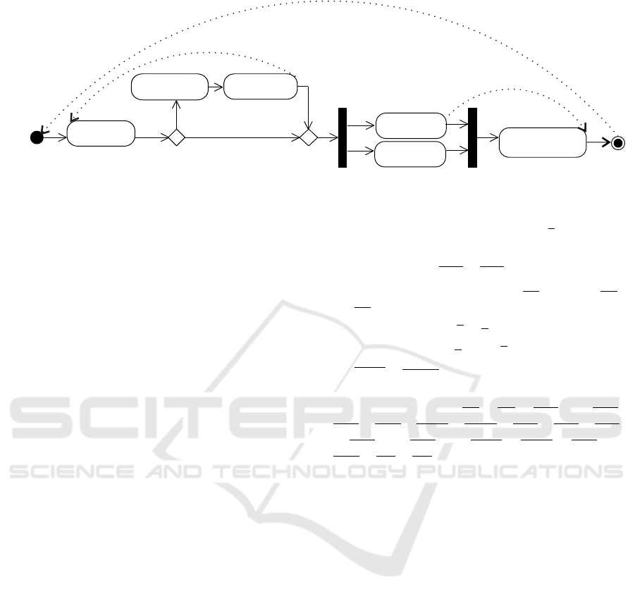
Figure 1 shows an example of an activity dia-

gram including temporal information. The example

describes a simpliﬁed and generic delivery service.

The activity starts when an order is received. The ﬁrst

step is the processing of the order information (A1)

which is modeled as a non-contingent action, lasting

between 1 and 2 minutes. After that, the agent per-

forming the activity, decides whether all information

is complete or not (C1). If there is something missing,

the customer has to be contacted and then, the pro-

cessing of the order information has to be completed

(A2 and A3). However, there is an upper-bound con-

straint requiring that the completion has to be done

at most 5 minutes after the initial processing of the

order information has started. The next two actions

A4 “Prepare Order” and A5 “Create Receipt” are per-

formed in parallel. “Prepare Order” is modelled as a

contingent action, which means that the actual dura-

tion cannot be controlled by the agent, and “Create

Receipt” is another non-contingent action lasting for

1 to 2 minutes. In addition, there is a lower-bound

constraint stating that the next action (A6) “Deliver to

Customer” ﬁnishes at least 15 minutes after the order

has been prepared. The action “Deliver to Customer”

is, itself, again modelled as contingent action, and

completes the whole activity. Because of the activity

deadline (visualized as dotted line from start action to

end action), the completion of the whole activity has

to take at maximum 30 minutes.

3 TEMPORAL ACTIVITY

MODEL

3.1 Formalizing Activity Diagrams with

Temporal Constraints

For most general applicability, here we introduce a

minimal model for designing temporal activity dia-

grams, which is sufﬁcient to capture the various tem-

poral information such as duration types and temporal

constraints.

We consider the most common control-ﬂow pat-

terns: sequence, decisions, splits, and the correspond-

ing joins. We consider action durations, activity dead-

line, and upper- and lower-bound constraints between

actions (start and end of actions). We measure time

in chronons, representing, e.g., hours, days, ..., en-

coded as natural numbers forming a time axis starting

at zero. A duration is deﬁned as the distance between

two time-points on the time axis.

We distinguish between non-contingent and con-

tingent actions. The duration of contingent actions

cannot be controlled; thus, it cannot be known when

they will actually terminate. The activity controller

may, however, control the duration of non-contingent

action at any time.

Deﬁnition 1 (Temporal Activity Model). An activity

A is a tuple (N, E, C, Ω), where:

• N is a set of nodes n with n.type ∈

{start, action, decision, split, join, end}. Each

n ∈ N is associated with n.s and n.e, the

start and end event of n. From N we derive

{n.s, n.e|n ∈ N}.

• E is a set of edges e = (n1, n2) deﬁning prece-

dence constraints.

• C is a set of temporal constraints:

– duration constraints d(n, n

min

, n

max

, dur) ∀n ∈

N, where n

min

, n

max

∈ N, dur ∈ {c, nc}, stating

that n takes some time in [n

min

, n

max

]. n can be

contingent (dur = c) or non-contingent (dur =

nc);

– upper-bound constraints ubc(a, b, δ), where

a, b ∈ N

, δ ∈ N, requiring that b ≤ a + δ;

– lower-bound constraints lbc(a, b, δ), where

a, b ∈ N

, δ ∈ N, requiring that b ≥ a + δ.

• Ω ∈ N is the maximum activity duration.

Time and Processes: Towards Engineering Temporal Requirements

A1: Process Order

Information [1,2]

A5: Create Receipt

[1,2]

A4: Prepare Order

[3,5] contingent

A6: Deliver to Customer

[1,6] contingent

A2: Contact Customer

[1,2]

A3: Complete Order

Processing [1,2]

C1j

C1: Information complete?

S: Receive Order

yes

Ω 30

LBC 15

P1j

UBC 5

Figure 1: Example of an activity diagram including temporal information.

3.2 Example Temporal Activity Model

Given the example described in section 2.1, we use

our model to formally describe the temporal require-

ments:

• N = {(S, start), (A1, action), (A2, action),

(A3, action), (A4, action), (A5, action),

(A6, action), (C1, decision), (C1 j, join),

(P1, split), (P1 j, join), (E, end)}

• E = {(S, A1), (A1,C1), (C1, A2), (C1, C1 j),

(A2, A3), (A3, C1 j), (C1 j, P1), (P1, A4),

(P1, A5), (A4, P1 j), (A5, P1 j), (P1 j, A6),

(A6, E)}

• C = {d(A1, 1, 2, nc), d(A2, 1, 2, nc),

d(A3, 1, 2, nc), d(A4, 3, 5, c), d(A5, 1, 2, nc),

d(A6, 1, 6, c), lbc(A4.e, A6.e, 15),

ubc(A3.e, A1.s, 5)}

• Ω = 30

It is easy to see that the formal model above cap-

tures the essence of the activity diagram. While the

activity diagram is much easier to communicate and

comprehend, the formal model is the basis for deﬁn-

ing the temporal semantics of the model formally and

to check the consistency, or correctness of a model

automatically.

3.3 Semantics of Temporal Activity

Models

We deﬁne the temporal semantics of temporal activity

models by deﬁning which scenarios are valid. A sce-

nario is an assignment of values to the events of the

activity model (starting and ending of actions), spec-

ifying when they occur. A scenario is valid, iff it sat-

isﬁes all temporal constraints.

Deﬁnition 2 (Valid Scenario). Let A(N, E,C, Ω) be

a temporal activity model. Let σ be a scenario for

A, assigning to each event e a value e. σ is a valid

scenario for P iff:

1. ∀(n1, n2) ∈ E, n1.e ≤ n2.s;

2. ∀d(n, n

min

, n

max

, [c|nc]) ∈ C, n.s + n

min

≤ n.e ≤

n.s + n

max

;

3. ∀ubc(a, b, δ) ∈ C, b ≤ a + δ;

4. ∀lbc(a, b, δ) ∈ C, a + δ ≤ b;

5. end.e ≤ start.s + Ω.

It is easy to see that the scenario for the process

in Figure 1 given by: S.s = S.e = A1.s = 0, A1.e =

C1.s = C1.e = C1 j.s = C1 j.e = P1.s = A4.s = A5.s =

1, A5.e = 2, A4.e = 5, P1 j.s = P1 j.e = A6.s = 13,

A6.e = E.s = E.e = 19 is valid.

A valid scenario represents an assignment of val-

ues to events, which does not violate any temporal

requirements. In the next section we discuss various

notions for deﬁning the avoidance of such violations.

4 CORRECTNESS OF

TEMPORAL REQUIREMENTS

4.1 Notions of Temporal Correctness

Engineering temporal requirements is not limited to

modeling temporal constraints. Indeed, a designer

must verify whether a set of temporal requirements

does not yield any contradictions, which would result

in the impossibility to fulﬁll all temporal constraints,

i.e. to temporal violations. So it is also part of the

requirements engineering the task of deﬁning when a

set of temporal requirements yields no contradictions.

Absence of contradictions is also known as temporal

correctness, and various deﬁnitions for it have been

proposed. We list here the most frequently adopted

notions, giving examples for each of them.

ICSOFT 2021 - 16th International Conference on Software Technologies

• Satisﬁability, also called consistency: it is the

most relaxed notion for temporal correctness. It

requires the existence of at least one valid scenario

satisfying all temporal constraints. However, it

admits the existence of other scenarios which are

not valid, i.e. for which some temporal constraint

is violated.

Example: the requirement “payment should be

completed within 2 days” for a money transfer

within the European Union is satisﬁable, since it

is possible that the bank completes the transfer in

2 days; however, it is also possible that the trans-

fer is completed in 3 or 4 days.

The above example shows that a violation may

occur, due to neglecting the uncertainty from the

contingent duration of the money transfer. Indeed,

the limitation of satisﬁability is that it does not

consider the possibility of uncontrollable (contin-

gent) durations, and assignments of conditions.

For this reason, satisﬁability is regarded as a weak

notion for temporal correctness.

• Strong Controllability: often a system may re-

quire a scenario to be valid for all possible con-

tingencies and observed conditions, with the ad-

ditional requirement that the assignments of val-

ues to events for such a scenario are independent

of contingencies and observed conditions. If it is

possible to ﬁnd such a valid scenario, then the sys-

tem is called strong controllable.

Example: the operations for a robot in a produc-

tion plan may need to be strictly scheduled in their

times of execution.

A scenario complying with strong controllability

may be, however, too restrictive and not always

be desirable, since it yields for all possible con-

tingent durations and observed conditions.

• Conditional controllability: it relaxes the require-

ment for a ﬁxed scenario independent of contin-

gent durations and conditions. It requires the ex-

istence of a valid scenario for each possible val-

ues of observed conditions. Hence, conditional

controllability allows for less restrictive scenarios

than strong controllability.

Example: assembling a machine components

must start no later than 2 days after receiving

them. However, shipping may be done with high

priority, taking 1 day, or with low priority, tak-

ing 4 days; in both cases shipping starts on the

same day. The time for starting assembly cannot

be ﬁxed independent of the shipping mode, other-

wise the constraint of starting within 2 days may

be violated.

Conditional controllability is less restrictive than

strong controllability. However, it may still re-

sult in too restrictive scheduling of events, or con-

straint violations, since it does not consider con-

tingent durations.

• Dynamic controllability: it requires the existence

of a scenario in which the values assigned to the

controllable time points may be based on smaller

assigned values, and that such a scenario is valid

for all possible contingent durations and observed

conditions.

Example:

a Nucleic Acid Ampliﬁcation Test

(NAAT) for SARS-CoV-2 may take from 1 hour

up to 24 hours to complete. Sending a SMS with

the NAAT result must be done at most 2 hours

after test completion. Clearly, the time for send-

ing the SMS cannot be ﬁxed before the NAAT is

completed, and it depends on the NAAT time of

completion.

Each of these temporal correctness notions may

be the most adequate in a given context. So speci-

fying the required temporal correctness notion is part

of the requirements speciﬁcation for a system. Next,

comes to problem of verifying whether such a require-

ment can be met, i.e. whether a corresponding valid

scenario can be achieved.

4.2 Checking Temporal Correctness

Major contributions to verifying temporal correct-

ness at system design time can be found in the ar-

eas of temporal logic (Alur and Henzinger, 1994;

Lamport, 1983) and Temporal Constraint Networks

(TCNs) (Dechter et al., 1991; Hunsberger, 2009).

Temporal logic focuses in particular on the tempo-

ral dependency relations such as before, during, and

after between events. TCNs, on the other hand, fo-

cus on the measured time distances between events

according to some time unit, which allows designers

a quantitative reasoning over temporal properties.

In essence, a TCN is a graph with nodes repre-

senting time points, and edges representing binary

constraints between time points in form of inequal-

ities. Reasoning approaches for checking temporal

correctness of TCNs are based on constraint propa-

gation, i.e. deriving implicit edges from the existing

ones, according to some rules. Deriving a negative cy-

cle (in the usual sense for graphs) through constraint

propagation signals the existence of a contradiction

between temporal constraints. On the other hand, if

constraint propagation for a TCN derives no negative

cycle, then the TCN yields no contradictions.

A broad number of TCN types have been pro-

posed and investigated, each offering a different level

Time and Processes: Towards Engineering Temporal Requirements

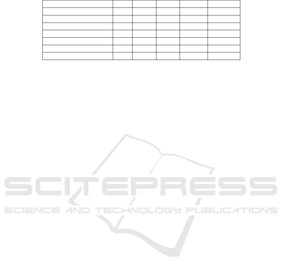
Table 1: Expressiveness comparison of various TCN types.

STN STNU CSTN CSTNU CSTNUD

non-contingent durations + + + + +

contingent durations + + +

parallel execution + + + + +

conditional alternative + + +

decisional alternative +

upper-bound constraints + + + + +

lower-bound constraints + + + + +

of expressiveness to meet different modeling require-

ments, and to support checking for different tempo-

ral correctness notions. We list here the major TCN

types:

• The Simple Temporal Network (STN) (Dechter

et al., 1991) is the simplest TCN type. In a STN all

time points can be assigned a value, and there are

no contingent durations or conditions. Thus, the

STN supports performing satisﬁability checks.

• The STN with Uncertainty (STNU) (Vidal and

Fargier, 1997) increases the expressiveness of the

STN with the possibility to represent contingent

durations. The STNU supports checking for con-

trollabilities.

• The Conditional STN (CSTN) (Tsamardinos

et al., 2003) increases the expressiveness of the

STN with the possibility to represent observed

conditions. Thus, it supports checking for various

types of controllabilities.

• The Conditional STN with Uncertainty (CSTNU)

(Hunsberger et al., 2012) combines the CSTN

with the CSTNU, allowing for the representation

of both observed conditions and contingent dura-

tions. Like the CSTN and STNU, the CSTNU

supports controllabilities checking procedures.

• The Conditional STN with Uncertainty and De-

cisions (CSTNUD) (Zavatteri and Vigan

o, 2019)

augments the capabilities of the CSTNU by dif-

ferentiating between observed conditionals and

decisions which may be taken by a controller.

Controllability checks for the CSTNUD are sup-

ported.

Table 1 summarizes the expressiveness of the ma-

jor TCN types, indicating the support of each TCN

type for representing different temporal constraint and

duration types, and various control ﬂow patterns.

Further research produced both additional TCN

types and extended process model with mappings to

TCNs, each catering for speciﬁc temporal require-

ments. Some examples of such extensions are:

• STNPSU (Lanz et al., 2015) to express partially

shrinkable uncertainty

• STNU with resources (Combi et al., 2019)

• STNU with temporal parameters (Franceschetti

and Eder, 2019)

• Activity models with temporal conditions for con-

trol structures (Pichler et al., 2017)

• Access controlled temporal networks ACTN

(Combi et al., 2017; Zavatteri et al., 2020)

• STNU with semi-contingent durations, i.e. dura-

tion can be controlled but only until an activity

starts (Franceschetti and Eder, 2021).

All these extensions to temporal constraint net-

works allow the extension of the modeling constructs

for extended activity diagrams without loosing the

possibility of checking the correctness of requirement

models.

For the example from Figure 1, an adequate

TCN for representing its temporal requirements is

the CSTNU, since it models contingent and non-

contingent durations, observed conditions, and upper-

and lower-bound constraints.

How can TCNs technically support checking tem-

poral correctness for a temporal activity model? Sev-

eral approaches make use of TCNs for checking tem-

poral correctness of process deﬁnitions, e.g., (Combi

and Posenato, 2009; Eder et al., 2019; Franceschetti

and Eder, 2019). These approaches are based on map-

ping rules which project the temporal requirements of

a process deﬁnition into a TCN. Basically, the rules

map each process event (start and end of tasks) into

a corresponding TCN node, and each temporal re-

quirement (durations, constraints) into a correspond-

ing TCN edge. Analogous mapping strategies can be

deﬁned for mapping the temporal requirements of a

temporal activity model into a TCN.

The resulting TCN subsumes the same set of sce-

narios subsumed by the temporal requirements of the

original process deﬁnition, i.e. they are temporally

equivalent. Thus, checking temporal correctness for

such a TCN realizes a check for temporal correctness

for the original process deﬁnition or activity model.

The algorithms for checking dynamic controlla-

bility have quite different complexity for the different

ICSOFT 2021 - 16th International Conference on Software Technologies

types of TCNs. Therefore, general checking proce-

dures ﬁrst analyze which concepts are used in a model

and then apply the appropriate checking algorithm.

Details of the different temporal constraint net-

works, the mapping of activity diagrams to the net-

works and the algorithms for checking dynamic con-

trollability of the networks and thus checking the cor-

rectness and consistency of the temporal requirements

are beyond the scope of this paper. We are only able

to give an overview about the different temporal con-

straint networks and which type of network supports

which type of control structures and temporal require-

ments together with pointers to the literature where

each of these networks and the algorithms are de-

scribed in detail.

5 CONCLUSIONS

Temporal constraints, goals and request are important

aspects in requirements engineering. Time-related

requirements have to be adequately elicitated, col-

lected, documented and represented in requirements

models and analyzed for correctness, consistency and

feasibility. We propose extensions of well-known

modeling techniques like UML activity charts with

rather intuitive concepts for expressing temporal re-

quirements. Recent advances in temporal constraint

networks allow mapping these models into different

kinds of temporal constraint networks, depending on

the features used in the requirements model. These

formal representations can apply recently developed

algorithms for checking correctness, consistency and

feasibility of temporal requirements.

We argue that this approach helps to close the gap

between popular modeling notations, which allow ex-

pressing only very basic temporal relationships and

the elaborated systems of temporal logic and temporal

automata for formally specifying temporal require-

ments which are often shunned by practitioners be-

cause of their formal challenges. Easily understand-

able and usable notions and their representation of

temporal requirements without losing the power and

rigor of reliable formal analysis of the properties of

requirements models is the goal of this research.

Here we only discussed core concepts of such ex-

tensions, but several other more advanced concepts

like temporal variables and parameters, temporal con-

ditions in control structures are available to further in-

crease the expressiveness of requirements models.

The integration of systems for representing re-

quirements with notions for representing temporal

constraints together with their formal apparatus will

open promising ways for managing temporal require-

ments and support improvements in addressing tem-

poral requirements throughout the software life cycle.

REFERENCES

Alur, R. and Henzinger, T. A. (1994). A really temporal

logic. Journal of the ACM (JACM), 41(1):181–203.

Cairo, M. and Rizzi, R. (2019). Dynamic controllability

of simple temporal networks with uncertainty: Sim-

ple rules and fast real-time execution. Theor. Comput.

Sci., 797:2–16.

Cheikhrouhou, S., Kallel, S., Guermouche, N., and Jmaiel,

M. (2015). The temporal perspective in business pro-

cess modeling: a survey and research challenges. Ser-

vice Oriented Computing and Applications, 9(1):75–

85.

Cimatti, A., Hunsberger, L., Micheli, A., Posenato, R., and

Roveri, M. (2016). Dynamic controllability via timed

game automata. Acta Informatica, 53(6-8):681–722.

Combi, C. and Posenato, R. (2009). Controllability in tem-

poral conceptual workﬂow schemata. In International

Conference on Business Process Management, pages

64–79. Springer.

Combi, C., Posenato, R., Vigan

o, L., and Zavatteri, M.

(2017). Access controlled temporal networks. In In-

ternational Conference on Agents and Artiﬁcial Intel-

ligence, volume 2, pages 118–131. SciTePress.

Combi, C., Posenato, R., Vigan

o, L., and Zavatteri, M.

(2019). Conditional simple temporal networks with

uncertainty and resources. J. Artif. Intell. Res.,

64:931–985.

Dechter, R., Meiri, I., and Pearl, J. (1991). Temporal con-

straint networks. Artiﬁcial intelligence, 49(1-3):61–

95.

Eder, J. and Franceschetti, M. (2020). Time and Busi-

ness Process Management: Problems, Achievements,

Challenges . In Mu

noz-Velasco, E., Ozaki, A., and

Theobald, M., editors, 27th International Symposium

on Temporal Representation and Reasoning (TIME

2020), volume 178 of Leibniz International Proceed-

ings in Informatics (LIPIcs), pages 3:1–3:8, Dagstuhl,

Germany. Schloss Dagstuhl–Leibniz-Zentrum f

ur In-

formatik.

Eder, J., Franceschetti, M., and K

opke, J. (2019). Control-

lability of business processes with temporal variables.

In Proceedings of the 34th ACM/SIGAPP Symposium

on Applied Computing, pages 40–47.

Eder, J., Franceschetti, M., and Lubas, J. (2020). Con-

ditional schedules for processes with temporal con-

straints. SN Computer Science, 1(4):1–18.

Eder, J., Panagos, E., and Rabinovich, M. (2013). Workﬂow

time management revisited. In Seminal contributions

to information systems engineering, pages 207–213.

Springer.

Franceschetti, M. and Eder, J. (2019). Checking temporal

service level agreements for web service compositions

with temporal parameters. In 2019 IEEE International

Time and Processes: Towards Engineering Temporal Requirements

Conference on Web Services (ICWS), pages 443–445.

IEEE.

Franceschetti, M. and Eder, J. (2021). Semi-contingent task

durations: Characterization and controllability. In Ad-

vanced Information Systems Engineering, 33rd Inter-

national Conference, CAiSE 2021, Melbourne, Aus-

tralia, 2021. In print.

Gross, A. and Doerr, J. (2009). Epc vs. uml activity dia-

gram - two experiments examining their usefulness for

requirements engineering. In 2009 17th IEEE Interna-

tional Requirements Engineering Conference, pages

47–56.

Hunsberger, L. (2009). Fixing the semantics for dynamic

controllability and providing a more practical charac-

terization of dynamic execution strategies. In 2009

16th International Symposium on Temporal Represen-

tation and Reasoning, pages 155–162. IEEE.

Hunsberger, L. and Posenato, R. (2020). Faster dynamic-

consistency checking for conditional simple temporal

networks. In Beck, J. C., Buffet, O., Hoffmann, J.,

Karpas, E., and Sohrabi, S., editors, Proceedings of

the Thirtieth International Conference on Automated

Planning and Scheduling, Nancy, France, October 26-

30, 2020, pages 152–160. AAAI Press.

Hunsberger, L., Posenato, R., and Combi, C. (2012). The

dynamic controllability of conditional stns with uncer-

tainty. arXiv preprint arXiv:1212.2005.

Koymans, R. (1990). Specifying real-time properties with

metric temporal logic. Real-time systems, 2(4):255–

299.

Lamport, L. (1983). What good is temporal logic? In IFIP

congress, volume 83, pages 657–668.

Lanz, A., Posenato, R., Combi, C., and Reichert, M. (2015).

Simple temporal networks with partially shrinkable

uncertainty. In International Conference on Agents

and Artiﬁcial Intelligence, volume 2, pages 370–381.

SCITEPRESS.

Laplante, P. A. (2017). Requirements engineering for soft-

ware and systems. CRC Press.

Macaulay, L. A. (2012). Requirements engineering.

Springer Science & Business Media.

Maler, O., Nickovic, D., and Pnueli, A. (2005). Real time

temporal logic: Past, present, future. In Interna-

tional Conference on Formal Modeling and Analysis

of Timed Systems, pages 2–16. Springer.

Parent, C., Spaccapietra, S., and Zim

anyi, E. (2006). Con-

ceptual modeling for traditional and spatio-temporal

applications: The MADS approach. Springer Science

& Business Media.

Pichler, H., Eder, J., and Ciglic, M. (2017). Modelling

processes with time-dependent control structures. In

International Conference on Conceptual Modeling,

pages 50–58. Springer.

Pichler, H., Wenger, M., and Eder, J. (2009). Composing

time-aware web service orchestrations. In Advanced

Information Systems Engineering, 21st International

Conference, CAiSE 2009, Amsterdam, The Nether-

lands, June 8-12, 2009. Proceedings, pages 349–363.

Tsamardinos, I., Vidal, T., and Pollack, M. E. (2003). Ctp:

A new constraint-based formalism for conditional,

temporal planning. Constraints, 8(4):365–388.

Van Lamsweerde, A. (2001). Goal-oriented requirements

engineering: A guided tour. In Proceedings ﬁfth IEEE

international symposium on requirements engineer-

ing, pages 249–262. IEEE.

Vidal, T. and Fargier, H. (1997). Contingent durations

in temporal csps: from consistency to controllabili-

ties. In Proceedings of TIME’97: 4th International

Workshop on Temporal Representation and Reason-

ing, pages 78–85. IEEE.

Wolper, P. (2000). Constructing automata from tempo-

ral logic formulas: A tutorial. In School organized

by the European Educational Forum, pages 261–277.

Springer.

Wondoh, J., Grossmann, G., and Stumptner, M. (2017).

Dynamic temporal constraints in business processes.

In Proceedings of the Australasian Computer Science

Week Multiconference, pages 1–10.

Young, R. R. (2004). The requirements engineering hand-

book. Artech House.

Zavatteri, M., Combi, C., Rizzi, R., and Vigan

o, L. (2020).

Consistency checking of stns with decisions: Manag-

ing temporal and access-control constraints in a seam-

less way. Information and Computation, page 104637.

Zavatteri, M. and Vigan

o, L. (2019). Conditional sim-

ple temporal networks with uncertainty and decisions.

Theor. Comput. Sci., 797:77–101.

Zavatteri, M. and Vigan

o, L. (2019). Conditional sim-

ple temporal networks with uncertainty and decisions.

Theoretical Computer Science, 797:77–101.

Zhou, Y., Maity, D., and Baras, J. S. (2016). Timed au-

tomata approach for motion planning using metric in-

terval temporal logic. In 2016 European Control Con-

ference (ECC), pages 690–695. IEEE.

ICSOFT 2021 - 16th International Conference on Software Technologies