Singularity Avoidance of Task-redundant Robots in Pointing Tasks: On

Nullspace Projection and Cardan Angles as Orientation Coordinates

Moritz Schappler

and Tobias Ortmaier

Institute of Mechatronic Systems, Leibniz University Hannover, An der Universität 1, 30823 Garbsen, Germany

Keywords:

Singularity Avoidance, Nullspace Motion, Task Redundancy, Parallel Robots, Euler Angles, Cardan Angles.

Abstract:

Robot manipulators are often deployed in tool-symmetric tasks, which only requires deﬁning end effector po-

sition and pointing direction. In this case six-axis serial industrial robots and full-mobility (spatial) parallel

robots have one degree of task redundancy. Using Cardan angles as orientation coordinates, a uniﬁed formu-

lation of the position-level and second-order inverse kinematics problem is set up for both robot types. An

efﬁcient scheme for difference-quotient approximation of gradients of performance criteria for projection into

the task redundancy’s nullspace is presented. The simulation example of a hexapod robot shows that avoiding

and exiting parallel robot singularities of type II is possible with the nullspace of all joints. The nullspace

controller scheme can be used in ofﬂine trajectory optimization and in online motion generation.

1 INTRODUCTION AND STATE

OF THE ART

Robot manipulators have been a subject of research

for decades. Still more complex parallel kinematic

machines (parallel robots), and more complex prob-

lems arise, such as mastering singularities and motion

in high-dimensional spaces. Due to their complexity,

these problems can only be solved with profound al-

gorithms and by the help of information technology.

The optimization of robots performing tasks with

axis-symmetric tools like arc welding (Huo and

Baron, 2008), drilling (Guo et al., 2015) or milling

(Mousavi et al., 2018) has gained increasing atten-

tion in research and industry over the last years. Due

to their workspace, serial robots are predestinated for

welding tasks but also for drilling tasks e.g. in the air-

craft industry. For machining tasks parallel robots are

favorable due to their higher stiffness than serial kine-

matic machine tools or serial robot arm manipulators.

Serial industrial robots as well as the hexapod par-

allel robot often used for machining tasks have six de-

grees of freedom (DoF) in the operational space and

in the (actuation) joint space. They do not have in-

trinsic redundancy (for serial robots) or kinematic or

actuation redundancy (in the case of parallel robots).

A task (or functional) redundancy of degree one ex-

https://orcid.org/0000-0001-7952-7363

https://orcid.org/0000-0003-1644-3685

ists, if the six-DoF robot is used in an axis-symmetric

task (requiring only ﬁve DoF). For a deﬁnition of the

redundancy see (Huo and Baron, 2008) or (Léger and

Angeles, 2016) for serial robots and (Gosselin and

Schreiber, 2018) for parallel robots.

The redundancy allows deﬁning a nullspace and

performing a pose optimization using gradient pro-

jection into that nullspace. This method is very ef-

ﬁcient and already well-established for kinematic re-

dundancy (Nakamura et al., 1987; Chiaverini et al.,

2008; Lillo et al., 2019). The redundancy of a rota-

tional end effector DoF requires the adaption of the

inverse kinematics problem (IKP) to account for the

nonlinearity of rotation. Further, the IKP can be dis-

tinguished between position level and velocity level

or higher differential order. Several geometric ap-

proaches for the IKP of task-redundant robots have

been investigated, such as

• twist decomposition (Huo and Baron, 2008),

• orthogonal decomposition of the task space

(Léger and Angeles, 2016; Corinaldi et al., 2016),

• reciprocal Euler angles (Schappler et al., 2019),

• separation of joint coordinates in redundant and

non-redundant on position level (Ozgoren, 2013)

or on velocity level (Reiter et al., 2018),

• expressing the end effector angular velocity in

the local frame and removing the last component

(Žlajpah, 2017; Reiter et al., 2018) corresponding

to the redundant coordinate.

338

Schappler, M. and Ortmaier, T.

Singularity Avoidance of Task-redundant Robots in Pointing Tasks: On Nullspace Projection and Cardan Angles as Orientation Coordinates.

DOI: 10.5220/0010621103380349

In Proceedings of the 18th International Conference on Informatics in Control, Automation and Robotics (ICINCO 2021), pages 338-349

ISBN: 978-989-758-522-7

The alternative to the modiﬁed inverse kinematics

(IK) formulations above is a full formulation of the

IK (ignoring task redundancy). Then, a subsequent

optimization of the redundant task space coordinate

is necessary, as performed by (Zhu et al., 2013), (Guo

et al., 2015) and (Mousavi et al., 2018) for serial

robots. Especially for parallel robots this approach

was previously pursued combined with

• interval analysis (Merlet et al., 2000),

• an iterative solution using linear or quadratic pro-

gramming (Oen and Wang, 2007),

• discrete switching patterns of the redundant coor-

dinate in rest positions (Kotlarski et al., 2010),

• iterations of small-angle perturbations of the re-

dundant coordinate (Gao et al., 2019).

In special variations of the milling task using par-

allel kinematic machines (PKM), more than one rota-

tional coordinate can be treated as redundant. Exam-

ples are end milling (Shaw and Chen, 2001) or milling

with a spherical cutter (Smirnov et al., 2013).

The overview already shows that gradient-based

local optimization approaches are more widely used

in serial robotics than in parallel robotics, where

global optimizations dominate. A promising strategy

is the combination of local and global approaches, e.g.

by using differential dynamic programming (Santos

and da Silva, 2017).

Only in recent publications, gradient-based opti-

mization with nullspace projection is performed for

parallel robots, with focus on kinematic redundancy

by (Gosselin and Schreiber, 2016) and (Santos and

da Silva, 2017) and on task redundancy by (Agarwal

et al., 2016). The main effort is put on the kinematic

and actuation redundancy, as can be seen in the ex-

tensive reviews on parallel robot redundancy (Luces

et al., 2017) and (Gosselin and Schreiber, 2018),

where task redundancy is not even mentioned.

Redundancy is exploited to improve performance

criteria of the robot manipulators, such as joint limits

(Huo and Baron, 2008; Zhu et al., 2013) or milling

process stability (Mousavi et al., 2018). Singularity

avoidance is implemented by criteria such as

• the distance in the joint space to the conﬁguration

that ﬁrst exceeded a parameter of singularity (Huo

and Baron, 2008),

• the squared condition number (Zhu et al., 2013;

Léger and Angeles, 2016; Corinaldi et al., 2016)

via the Frobenius norm relation (Merlet, 2006),

• the condition number of the PKM forward kine-

matics Jacobian (Gosselin and Schreiber, 2016),

• the consideration of all singular values of the Ja-

cobian (Santos and da Silva, 2017),

• the homogenized pose error as a measure for ac-

curacy and singularities (Kotlarski et al., 2010),

• the Jacobian’s determinant (Agarwal et al., 2016).

Although the physical meaning of the manipula-

tor Jacobian’s condition number is questionable, cf.

(Kotlarski et al., 2010), using it as a measure for sin-

gularity avoidance is well established and can be justi-

ﬁed, even without homogenization of units, cf. (Mer-

let, 2006). Especially for parallel robots singulari-

ties can be located anywhere in the workspace and

avoiding them in ofﬂine trajectory planning and on-

line trajectory execution is paramount, cf. (Luces

et al., 2017; Gosselin and Schreiber, 2018).

The work from (Agarwal et al., 2016) presents

a promising approach to tackle the problem of sin-

gularity avoidance for parallel robots using gradient

projection in the nullspace of task redundancy. How-

ever, open points remain, regarding the feedback loop

design of the nullspace motion and an extension to

spatial robots regarding the nonlinearity of rotation.

These points will be encountered in this paper by a

consideration of Cardan angles as end effector coor-

dinates, as in (Schappler et al., 2019), by considering

a second-order nullspace motion, cf. (Reiter et al.,

2018) and by incorporating aspects of control design

from (De Luca et al., 1992), where this problem was

already approached for serial robots. To summarize,

the contributions of this paper are

• a formulation of the differential inverse kinemat-

ics problem for one-DoF task redundancy using

Cardan angles for end effector orientation,

• a numeric scheme for simpliﬁcation of the com-

putation of gradients of performance criteria in the

nullspace projection using difference quotients,

• unifying the scheme for serial and parallel robots,

• and exemplary simulative studies on ofﬂine tra-

jectory planning with singularity avoidance.

The remainder of the paper is structured as fol-

lows. After a remark on task coordinates in section 2,

the kinematics model and nullspace motion is laid out

in section 3 for serial robots and in section 4 for paral-

lel robots. Considerations on the control loop design

and remarks on convergence are given in section 5

and the scheme is validated in section 6 at the exam-

ple of pose optimization and trajectory tracking of a

six-DoF parallel robot. Section 7 concludes the paper.

2 ON TASK COORDINATES

In the following, the six operational space coordi-

nates, i.e. the position and orientation of a robot’s end

effector in the Cartesian space, are expressed with the

vector x

x = (r

,ϕ

)

. Unlike for the un-

ambiguous position part r

r, a suitable representation

of rotation has to be chosen for the orientation part ϕ

ϕ.

Singularity Avoidance of Task-redundant Robots in Pointing Tasks: On Nullspace Projection and Cardan Angles as Orientation Coordinates

339

For tasks with rotational symmetry given in sec-

tion 1, a selection of the Euler angle convention is

suitable, where the last of the three (intrinsic) elemen-

tary rotations is deﬁned around the tool axis. The

Cardan angles (or X -Y ’-Z” Euler angles) are espe-

cially practical and intuitive, since the tool axis in

robotics is by convention the z

-axis. The end ef-

fector’s rotation matrix w.r.t. the base frame is de-

ﬁned by

x) = R

(ϕ

) using the ba-

sic rotation matrices. The angle convention estab-

lished in tool machines on the contrary follows the

extrinsic X -Y -Z Euler angles convention for express-

ing orientation, which corresponds to the intrinsic

Z-Y ’-X ” convention. The rotation axes are termed

“A, B and C” (corresponding to “X, Y and Z” transla-

tion), (Smirnov et al., 2013). The term “Euler angles”

is used for generalization, also including Tait-Bryan

(and Cardan) angles and is not limited to proper Eu-

ler angles. Representing orientation with Euler angles

can introduce mathematical singularities correspond-

ing to a gimbal lock. For Cardan angles this only

occurs for ϕ

=±90

◦

, which is not relevant for most

tasks and e.g. technically not possible for most paral-

lel robots and therefore out of this paper’s scope.

The task space coordinates of pointing tasks are

deﬁned as y

y = (r

,ϕ

)

. Due to the rota-

tional symmetry of the robot tool and the chosen rep-

resentation of rotation, the last operational space co-

ordinate ϕ

corresponds to a rotation of the robot end

effector around the tool axis and can be selected arbi-

trarily in the regarded case of task redundancy.

3 SERIAL-LINK ROBOTS

Redundancy resolution for serial robots has been

widely researched, cf. (Chiaverini et al., 2008), but

the case of task redundancy is only implicitly in-

cluded in the fundamental works. In the following,

section 3.1 clariﬁes some foundations e.g. from (Chi-

averini et al., 2008) regarding task redundancy and

section 3.2 introduces new aspects on the computa-

tion of the nullspace in task redundancy.

3.1 Inverse Kinematics Model

The forward kinematics problem relates the n

joint

space coordinates q

q with the operational space by

x =



, x





q), ϕ

XY Z

(

q))



. (1)

The non-redundant inverse kinematics problem (IKP)

can be expressed by an implicit residual in R

Φ(q

q,x

x) =





−x

+ r



)



= 0

0 (2)

with arbitrary convention θ

θ, which can be solved nu-

merically using the Newton-Raphson algorithm. In

the case of task redundancy, a reduced residual

Ψ(q

q,y

y) = 0

0 ∈ R

with rotational part (3)



0 1 0

0 0 1



ZY X



)



∈ R

(4)

is needed, which can be set up by using the Euler an-

gles θ

θ of the rotation matrix between desired pose x

and actual pose x

x(q

q). The angle convention in Ψ

Ψ has

to be reciprocal (i.e. Z-Y ’-X”) to the one used for the

end effector pose x

x, as derived in (Schappler et al.,

2019). The redundant coordinate ϕ

has no effect.

Using a task-redundant robot with n

≥ 6 allows

to optimize additional objective functions h(q

q) using

nullspace projection in the iterative solution by

opt

= argmin

(h(q

q)) s.t. Ψ

Ψ(q

q,y

y) = 0

0. (5)

The iterative solution in the step k is obtained with

the Moore-Penrose pseudo-inverse by

k+1

= q

− Ψ

∂q

Ψ + (I

− Ψ

∂q

)(−h

∂q

), (6)

where the index ∂q

q denotes the derivative of the sym-

bol w.r.t. q

q, # the pseudo-inverse, I

the identity ma-

trix of appropriate dimension n

and the dependency

on q

and y

y is omitted for the sake of brevity. The

notation will be kept throughout the paper.

Using this allows to optimize the robot for one

speciﬁc pose, e.g. for drilling tasks, where the feed

motion is negligible regarding the robot’s dimension.

To obtain a continuous trajectory, e.g. for milling

tasks, the forward differential kinematics

x = J

q and

x =

q + J

q (7)

are used. The matrix J

is known as the analytic Jaco-

bian. The geometric Jacobian on the contrary relates

angular velocities in the base frame instead of time

derivatives of the Euler angles to the joint velocities.

The transfer from operational space to task space

is performed by removing the last row of (7) with

y = P

x and J

= P

. The matrices J

and Ψ

∂q

are not identical due to the nonlinearity of rotation in

SE(3). The task space inverse differential kinematics

are obtained by the pseudo-inverse solution

q =

= J

(

y −

q) + (I

− J

v. (8)

Again as in (6), nullspace projection of arbitrary vec-

tors v

v can be performed. The vector may be chosen as

v = −h

∂q

or as discussed in section 5.

3.2 Task Redundancy and Nullspace

Objective functions h(q

q) can be deﬁned analytically

or numerically. The former is not possible or feasible

for all functions. For the latter a method for the efﬁ-

cient derivation of the gradient h

∂q

will be presented

and discussed for several cases.

ICINCO 2021 - 18th International Conference on Informatics in Control, Automation and Robotics

340

3.2.1 General Case

The general case is not limited to task redundancy and

can be used in the position-level inverse kinematics

problem (6) for kΨ

Ψk 6≈ 0. A difference quotient is

calculated for a small increment ∆q

of all joints by

∂q

≈ (h(q

q + ∆q

q) − h(q

q))/∆q

, (9)

where ∆q

= 0 with j 6= i in ∆q

q. This requires n

evaluations of the objective function h(q

q) in each iter-

ation of (6) or each discrete trajectory sample of (8).

This is e.g. mentioned in (Lillo et al., 2019), but is

probably used in many implementations.

3.2.2 Task Redundancy of Degree One

In the case of task redundancy with n

−dim(y

y) = 1,

the nullspace projection can be exploited to simplify

the computation. The assumption is that kΨ

Ψk ≈ 0,

which is always the case in the differential inverse

kinematics (8). In the position-level IKP (6) conver-

gence of the task or an already valid initial value q

required. Writing q

q := q

q(x

x) leads to

∂h

∂x

∂h

∂q

∂x

∂h

∂q

∂h

∂x

∂q

. (10)

The latter expression can be divided into the single

operational space coordinates via

∂h

∂q

∂h

∂r

∂q

∂h

∂r

∂q

+ ... +

∂h

∂ϕ

∂q

. (11)

The nullspace projector included in (6) or (8) is

N = I

−J

= I

−Ψ

∂q

for kΨ

Ψk = 0. (12)

Since the nullspace is deﬁned as a rotation within the

coordinate, the projector eliminates the other terms



∂h

∂r

∂q



= 0

0, ..., N



∂h

∂ϕ

∂q



= 0

0. (13)

Therefore the gradient in the case of one-DoF task

redundancy can be simpliﬁed to

∗

∂q

∂h

∂ϕ

∂q

, (14)

where the last term is the last row of the Jacobian J

The asterisk denotes the simpliﬁed calculation of the

gradient which follows the relations

N(h

∗

∂q

)

= N

N(h

∂q

)

and h

∗

∂q

6= h

∂q

. (15)

Using a small increment of the redundant coordinate

∆x

x = (0

,∆ϕ

)

, the ﬁrst term can be determined nu-

merically via the difference quotient

(∂h/∂ϕ

) ≈ (h(q

q + J

−1

∆x

x) − h(q

q))/∆ϕ

. (16)

This only requires two numeric evaluations of h(q

which can be highly beneﬁcial for computationally

expensive objectives such as collision avoidance or

singularity avoidance. The approach of simulating

a ∆ϕ

can be regarded similar to the principle of

small-angle perturbation of (Gao et al., 2019), where

a global instead of local optimization is performed.

4 PARALLEL ROBOTS

The inverse kinematics of task redundant parallel

robots can be approached similarly as serial robots.

A a parallel robot consists of m kinematic chains con-

necting a base link with a moving platform. Follow-

ing e.g. (Merlet, 2006), the joint space q

q now also

contains passive joints (here also including the plat-

form coupling joints). Active joint coordinates are in-

cluded in this formulation and are also denoted by θ

θ.

Further, the platform pose can be expressed by the op-

erational space coordinate x

x which can also be used as

a minimal coordinate of the robot.

In the following, section 4.1 again applies ap-

proaches from literature, e.g. (Merlet, 2006; Chi-

averini et al., 2008) to task redundancy and section 4.2

discusses projection in the nullspace.

4.1 Inverse Kinematics Model

To solve the IKP for parallel robots, similar to (2)

and (3) for serial robots, the full and reduced kine-

matic constraints Φ

Φ(q

q,x

x)∈R

and Ψ

Ψ(q

q,y

y)∈R

6m−1

are deﬁned. The latter can be obtained in the mini-

mal form only dependent on the task space coordinate

y by using reciprocal Euler angles for the orientation

constraints of the ﬁrst leg chain like in (4). The con-

straints of other (following) legs are deﬁned relative

to the ﬁrst (leading) leg, e.g. as vector loop via the

end effector, see (Schappler et al., 2019). While the

IKP can be solved with the same Newton-Raphson

approach (6) as serial robots, the differential relation

∂q

q + Φ

∂x

x = 0

0 and Ψ

∂q

q + Ψ

∂y

y = 0

0 (17)

also has to take the platform coordinates x

x and accord-

ingly y

y into account. The inverse differential kine-

matics is split up into the particular solution and the

nullspace solution by

q =

. The task-related

differential inverse kinematics on velocity level is

= −Φ

−1

∂q

∂x

x =

−1

x. (18)

The matrix

−1

is the Jacobian relating all joint veloc-

ities and the platform velocity (in operational space

coordinates x

x). The acceleration can be obtained by

−1

x +

−1

x. (19)

Singularity Avoidance of Task-redundant Robots in Pointing Tasks: On Nullspace Projection and Cardan Angles as Orientation Coordinates

341

In the case of task redundancy, either the solution of

(19) with

=0 can be selected or the minimum-

norm solution by using the Ψ

Ψ-related constraints with

= −Ψ

∂q



∂q

q +

∂y

y + Ψ

∂y



. (20)

Another approach is obtaining

from time differ-

entiation of

= −Ψ

∂q

∂y

y, which was shown for

serial robots by (Reiter et al., 2018). Similar to (8),

the nullspace motion in the full joint space on accel-

eration level is obtained as

= (I

− Ψ

∂q

. (21)

It has to be noted that for the full joint space of par-

allel robots a relation of the nullspace projector and

the Jacobian like (12) for serial robots does not exist

directly. Only the inverse matrix

−1

can be deﬁned,

but not the non-inverse

, since n

> dim(x

x).

To be able to use the manipulator Jacobian J

for

the nullspace projection, the nullspace motion has to

be computed in the actuation space with n

coordi-

nates θ

θ. This can be obtained by selection of compo-

nents of the full joint space expressions with

θ = P

q and J

−1

= P

−1

. (22)

The manipulator Jacobian can be computed by (nu-

meric) matrix inversion with



−1



−1



−1



−1

. (23)

Only after this step, the reduced Jacobian J

without

the row for the redundant task space coordinate ϕ

can

be obtained analogously to the serial robot case with

= P

. This approach does not require a minimal

kinematics set, where passive joints are eliminated in

the constraints resulting to Φ

Φ(θ

θ,x

x) instead of Φ

Φ(q

q,x

x),

like e.g. used by (Agarwal et al., 2016).

Actuator speeds

θ can be projected in the full joint

space by

q =

−1

θ. (24)

The nullspace motion can then be computed like

in the serial robot case (8) with

= J

(

y−

θ) and

= (I

−J

. (25)

The two nullspace formulations lead to the same

motion and combining (24) with (25) and (21) lead to

the relation

= k

−1

−T

(26)

with N

= I

− Ψ

∂q

and N

= I

− J

. The

relation of the scalar factor k = k(q

q) is yet to be found.

The structure of the nullspace of task redundancy is

visible in the term J

, where only the last scalar

entry is non-zero, corresponding to a motion in the co-

ordinate ϕ

. The serial robot case of (12) is included

in (26) by the relation

−1

= I

I due to n

= n

Obtaining the matrix J

requires the inversion of

∂q

in (18). If the matrix is rank deﬁcient, a singular-

ity of type I is present. More critical are singularities

of type II, where Φ

∂q

has full rank but J

−1

has not.

This is caused by the structure of Φ

∂x

and the choice

of actuated joints by P

, cf. (Merlet, 2006).

4.2 Task Redundancy and Nullspace

The main difference between nullspace motion for

serial and parallel robots is the existence of the full

joint space different from the actuation joint space,

i.e. P

6= I

I. As discussed above, the nullspace projec-

tor for the full joint space only relies on the geometric

matrix of the inverse kinematics Ψ

∂q

and not on the

Jacobian J

. Therefore this coordinate space is es-

pecially suitable to generate desired motion although

being in or near a singularity of type II. Further, it can

be used to incorporate objective functions h(q

q) e.g.

for the joint limits of passive joints. Several cases can

be distinguished:

4.2.1 General Case (Position-level IKP)

The general case is similar to section 3.2.1 for serial

robots. This case is useful especially if kΨ

Ψk 6≈ 0, like

in the position-level IKP. For parallel robots with ob-

jectives h(q

q) only dependent on the joint coordinates

it is identical to serial robots. For criteria h(q

q,x

x),

∂q

≈ (h(q

q + ∆q

q,x

x) − h(q

q,x

x))/∆q

(27)

is used, with ∆q

= 0 for j 6= i. This corresponds to the

quotient from (9). No change of x

x is considered, since

by kΨ

Ψk 6≈ 0 the kinematic loops of the robot are not

closed with the platform. In the case of a full-mobility

parallel robot, n

= 36 and therefore the n

+1 evalu-

ations become computationally expensive.

4.2.2 Task Redundancy and Full Joint Space

In the case that the kinematic constraints are met,

kΨ

Ψk ≈ 0 holds and the preceding approach is not ef-

ﬁcient. Nullspace motion and objective function are

deﬁned in the full joint space like v

= −(∂h/∂q

The one-DoF task redundancy can be exploited by

consideration of the elimination of components with

the nullspace projector as in (13). The nullspace mo-

tion in operational space ∆x

x=(0

,∆ϕ

)

results in the

full joint space to ∆q

q =

−1

∆x

x. With this, the numeric

approximation of the gradient for task redundancy is

∗

∂q

≈ (h(q

q + ∆q

q,x

x + ∆x

x) − h(q

q,x

x))/∆q

. (28)

ICINCO 2021 - 18th International Conference on Informatics in Control, Automation and Robotics

342

The nullspace motion is obtained by the projector

= I

− Ψ

∂q

∈ R

×n

from (21). The formu-

lation requires only two evaluations of h(q

q,x

x).

4.2.3 Task Redundancy and Actuation Space

Computing the nullspace motion in the actuation joint

space with v

= −(∂h/∂θ

θ)

has the advantage of only

using the projector N

= I

− J

∈ R

×n

from

(25) of much lower dimension than in the previous

scheme, since e.g. n

=6 and n

=36 for fully parallel

robots. The assumption kΨ

Ψk ≈ 0 still has to hold.

The approach (14) from the serial robot case can

be adapted to the parallel robot objective function

h(q

q,x

x), similar to the procedure leading to (28). An-

ticipating the nullspace projection, as a ﬁrst step, the

gradient is projected from the redundant coordinate

into the actuated joint space with

∗

∂θ

∂h

∂ϕ

∂θ

. (29)

Numeric approximation of the ﬁrst gradient yields

(∂h/∂ϕ

) ≈ (h(q

q + ∆q

q,x

x +∆x

x)−h(q

q,x

x))/∆ϕ

. (30)

The second term of (29) again is the last row of J

which requires the inversion (23) and therefore a non-

singular conﬁguration of the robot. If the trajectory

is generated for the full joint space, then the actuator

nullspace motion

= N

can be projected in that

space by the time derivative of

−1

If the gradient ∂h/∂q

q is available in analytic form,

the projection can be performed by

∂h

∂θ

∂h

∂q

∂θ

∂h

∂q

−1

. (31)

This is helpful if e.g. the function for hyperbolic dis-

tance to the joint limits from (Zhu et al., 2013) is used.

5 NULLSPACE MOTION

The previous two sections review different modalities

for nullspace motion of serial and parallel robots. The

focus is on the necessary gradients of objective func-

tions h in the case of task redundancy. The schemes

(8), (21) and (25) are deﬁned on acceleration level.

This allows to generate a consistent and continuously

differentiable trajectory of q

q(t),

q(t) and

q(t), which

is beneﬁcial for the implementation for tracking con-

trollers with feed-forward control with inverse dy-

namics, cf. (De Luca et al., 1992) and (Reiter et al.,

2018). A general nullspace vector v

v is used in the

equations of this paper, which allows incorporating

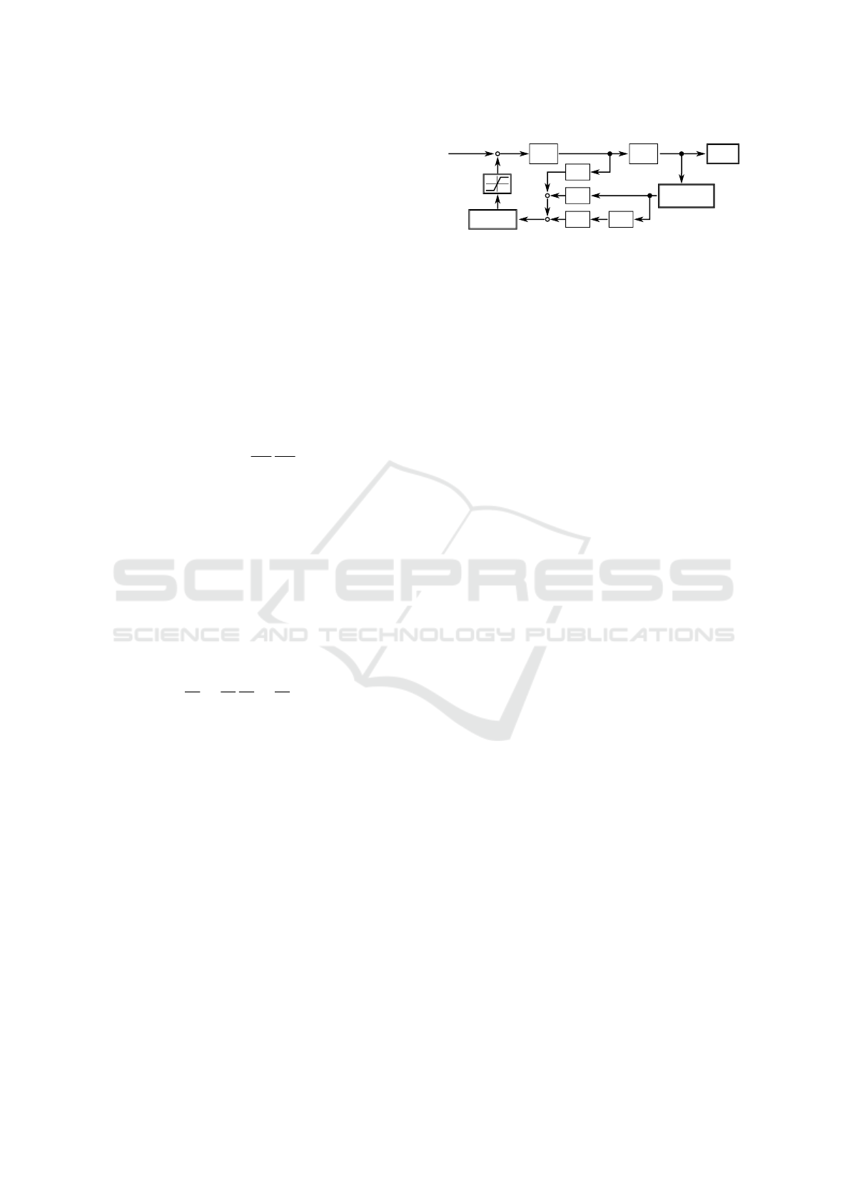
different control architectures. A general architecture

q q

h(q

N(q

q)v

−h

∂q

/dt

Figure 1: Nullspace motion controller scheme.

from (De Luca et al., 1992) is depicted in Figure 1. It

uses a nullspace feedback loop with a PD controller

and K

) and an additional damping term (K

The architecture can be applied in all cases presented.

As stated in (Reiter et al., 2018), using the

nullspace component in the differential kinematics on

acceleration level is not equivalent to the derivative of

the velocity-level solution. One approach is to per-

form analytic differentiation of the nullspace scheme,

which works for serial robots up to higher orders (Rei-

ter et al., 2018). Since this may be computational ex-

pensive for parallel robots, a discrete time implemen-

tation for the differentiation is used here, as suggested

by (De Luca et al., 1992). Therefore the projection

schemes on acceleration level of (8) and (21) do not

fall into the non-equivalence category explained by

(Reiter et al., 2018), if used as depicted in Figure 1.

Resolution of task redundancy on acceleration

level with nullspace projection was introduced for

parallel robots by (Agarwal et al., 2016), There only

v= −K

∂θ

is used, which corresponds to K

in Figure 1. In that reference, a proof of stability of

this control strategy was performed stating that the

potential h is never increasing (in the minimization

case). Due to the assumption

q= 0

0 which was ex-

tended from the initial value to generality, the proof

is only valid for h(t=0), not for h(t>0) and the state-

ment can not be supported by the proof as shown next.

The nonlinear control system of Figure 1 can be

described as a multi-input, multi-output system with

nonlinear input gain N

N(q

q) and output function h

∂q

and a double integrator as internal dynamics, neglect-

ing the task tracking input

and the limitation of

Already in the linear case, controlling a double inte-

grator system only with proportional feedback leads

to undamped oscillations. A stabilizing control is pos-

sible using a PD controller structure. This consider-

ation leads to a use of all gains, K

> 0, as

suggested in (De Luca et al., 1992).

The derivative gain K

leads to high values for

the nullspace acceleration when not already starting

in an optimum of h – exactly like the velocity-based

schemes this corresponds to. Therefore, an additional

limit is added into the control scheme of Figure 1,

with

N,max

max

−

. This presents an alternative

to the successive consideration of maximum acceler-

Singularity Avoidance of Task-redundant Robots in Pointing Tasks: On Nullspace Projection and Cardan Angles as Orientation Coordinates

343

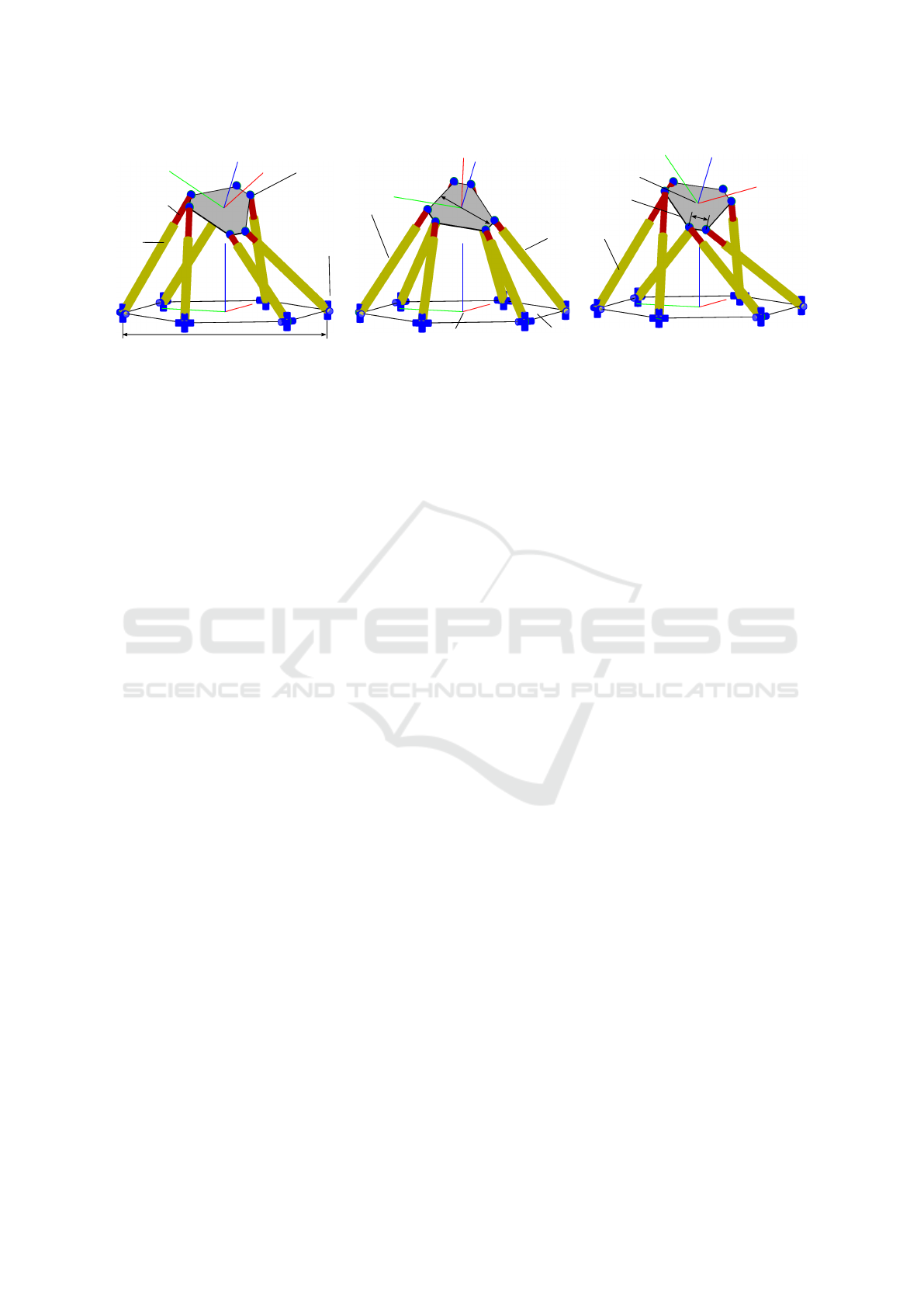
(a) initial pose case 1

prismatic joint

universal joint

moving platform

base platform (symmetric)

(lift cylinder)

leg chain

spherical joint

end effector frame (CS)

base frame (CS)

(b) initial pose case 2 (singular) (c) ﬁnal pose (both cases)

◦

, cond(J

−1

)=107.5 ϕ

=33.8

◦

, cond(J

−1

)=1.8· 10

=−25.0

◦

, cond(J

−1

)=56.1

extensible

cylinder

outer

cyl.

Figure 2: Task-redundant poses of the parallel robot of Sec. 6.1: (a) non-singular pose, (b) singular pose, (c) ﬁnal value.

ations in the velocity-based schemes like (Santos and

da Silva, 2017). Additional nullspace motion is gen-

erated to counteract when approaching limits q

max

joint positions and

max

of joint velocities. Lower

limits q

min

are handled in the same manner.

The amount and extent of objectives that can be

included in the task redundancy resolution scheme is

limited if only one degree of redundancy exists. In-

stead of a nested nullspace projection like in (Naka-

mura et al., 1987), only weighted sums of objectives

can be used, which can be sufﬁcient for properly de-

signed objective functions as in (Zhu et al., 2013) or

when prioritizing objectives, cf. (Lillo et al., 2019).

6 CASE STUDY

The validation of the nullspace projection of section 4

and the controller scheme of section 5 is performed

in the following via simulation. The assumption of a

ﬁve-DoF task and a six-DoF robot still holds. A paral-

lel robot is used since the beneﬁts and applicability of

the proposed methods are better than for serial robots.

6.1 Singularity Avoidance in Nullspace

The nullspace motion is ﬁrst examined without an ad-

ditional robot task motion, i.e.

= 0

0. The pre-

sented method can be applied to optimize any scalar

performance criterion h in the nullspace of the task

redundancy. In this example, the condition number

of the robot Jacobian matrix of (23) is selected as

h(q

q,x

x) = cond(J

) = cond(J

−1

). Minimizing this cri-

terion moves the manipulator towards low condition

numbers and therefore away from singularities.

A hexapod parallel (Stewart-Gough type) robot is

considered in a pose y

y with a high tilting angle of the

platform. Technical details of the robot are given in

Table 1. The high tilting angle (expressed by ϕ

and

) presents the general spatial case, where the repre-

sentation of orientation by Cardan angles (X-Y ’-Z”)

is beneﬁcial. The torsion angle ϕ

of the platform is

set to two different values, depicted in Fig 2 a and 2 b,

representing the two cases to be investigated.

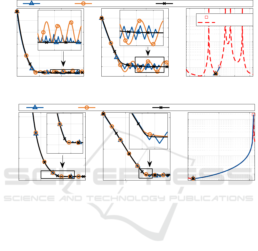
6.1.1 Case 1: Non-singular Initial Pose

In the ﬁrst case the robot starts in the non-singular

pose of Fig 2 a with ϕ

z,start,1

◦

. The values of the

optimization objective h over the redundant coordi-

nate ϕ

are depicted in Figure 3 c over a full rota-

tion of the platform (red dashed line). The over-

all performance of the robot is highly inﬂuenced by

singularities, which are located at ϕ

z,sing,1

≈−65

◦

z,sing,2

≈34

◦

, ϕ

z,sing,3

≈64

◦

and ϕ

z,sing,4

≈136

◦

. The

locations of these singularities ϕ

z,sing

were obtained

from global evaluation of the redundant coordinate.

The nullspace motion is ﬁrst generated by the

position-level IK scheme of (6). The convergence to-

wards the next local minimum of h(ϕ

z,ﬁnal

)=56.1 at

z,ﬁnal

=−25

◦

can be comprehended from Fig 3 a for

h(t), from Fig 3 b for ϕ

(t) and from Fig 3 c for the

characteristic diagram h(ϕ

) (blue lines). Compared

to the initial value of h(ϕ

z,start,1

)=107.5 it can be as-

sumed that the overall performance of the robot is im-

proved by the nullspace motion. This could be quanti-

ﬁed by other, more physically motivated performance

criteria such as accuracy, stiffness or actuator forces,

but is out of scope of this publication. The position-

level scheme only serves as a reference, since no time

relation is included originally and the steps k of (6)

are transferred to a time basis t using the joint velocity

limits. A C

-continuous trajectory (with continuously

differentiable position and velocity) regarding limits

for

q and

q can not be assured by this.

Therefore, the nullspace motion is obtained using

the trajectory IK scheme from (25) and section 4.2.3

ICINCO 2021 - 18th International Conference on Informatics in Control, Automation and Robotics

344

-180 -90 0 90 180

in deg

h = cond(J

)

(c)

initial value

computed offline

0 1 2 3

time in s

-30

-25

-20

-15

-10

-5

in deg

(b)

position-level IK trajectory IK with K

= K

= 0 traj e ctory IK with tuned gains

0 1 2 3

time in s

100

110

h = cond(J

)

(a)

Figure 3: Simulation results of the parallel robot starting in the non-singular pose from Fig 2 a.

-30 0 30

in deg

h = cond(J

)

(c)

0 1 2 3

time in s

-30

in deg

(b)

position-level IK trajectory IK with gain set 1 trajectory IK with gain set 2

0 1 2 3

time in s

100

150

200

h = cond(J

)

(a)

Figure 4: Simulation results of the parallel robot starting in the singular pose from Fig 2 b.

in the actuator space. To emphasize the argumenta-

tion of section 5, ﬁrst the feedback gains K

= 0 and

= 0 are used with K

= 1. A discrete-time imple-

mentation with sample time 1 ms was used. The time

evolution in Fig 3 a and 3 b shows undamped oscilla-

tions (orange lines). Therefore this parameterization

does not allow to reach the purpose of moving to the

next local optimum of h with little overshoot and fast

convergence. To accomplish this control objective,

the parameterization K

=0.5, K

=1 and K

=0.5 is

selected, which was obtained by manual tuning. The

motion controller now reaches the optimal value of

z,ﬁnal

=−25

◦

within about two seconds (black lines).

6.1.2 Case 2: Singular Initial Pose

The proposed new nullspace projection approach

of the full joint coordinate space of (21) and sec-

tion 4.2.2 has to be used if the initial pose or an

intermediate pose represents a singular conﬁgura-

tion. This is the case for the second starting pose

z,start,2

=33.8

◦

, where a numeric value for the con-

dition number of cond(J

−1

) = 1.8 · 10

is reached. In

this case, the inversion of J

−1

is not possible (or at

least does not produce feasible results). Controller

schemes relying on J

, e.g. formulated in the op-

erational space, would produce high accelerations or

high actuator forces. Therefore a controller scheme

avoiding this drawback has to be used as a fallback

to physically operate the robot, e.g. a scheme deﬁned

only in the actuator space.

The motion controller of section 5 is again used to

generate the nullspace motion with singularity avoid-

ance, as in the previous case. This time, the motion

is generated in the full joint space from (21) and sec-

tion 4.2.2 with the trajectory IK scheme.

The simulation results are given in Fig 4. Again,

the position-level IK and two parameterizations of the

trajectory IK are shown, while the position-level IK

only serves as comparison. The gains for the tra-

jectory IK were tuned manually and using a parti-

cle swarm optimization and were set to K

=0.03,

=0.01, and K

=0.05 in the ﬁrst set and K

=0.2,

=0.03 and K

=0.5 in the second set. With both

sets again a fast convergence within two seconds can

be achieved while maintaining the limits for q

q and

Singularity Avoidance of Task-redundant Robots in Pointing Tasks: On Nullspace Projection and Cardan Angles as Orientation Coordinates

345

0 1 2 3 4 5 6 7

Normalized trajectory progress s (per point of support)

-100

-50

100

150

Redundant c oordinate '

in deg

(a)

100

150

200

250

300

350

400

Performance criterion (condition number, joint limits)

ref. set 1 set 2 set 3 set 4

0 1 2 3 4 5 6 7

Norm. traje c t or y progress s

100

150

200

300

400

500

600

(b)

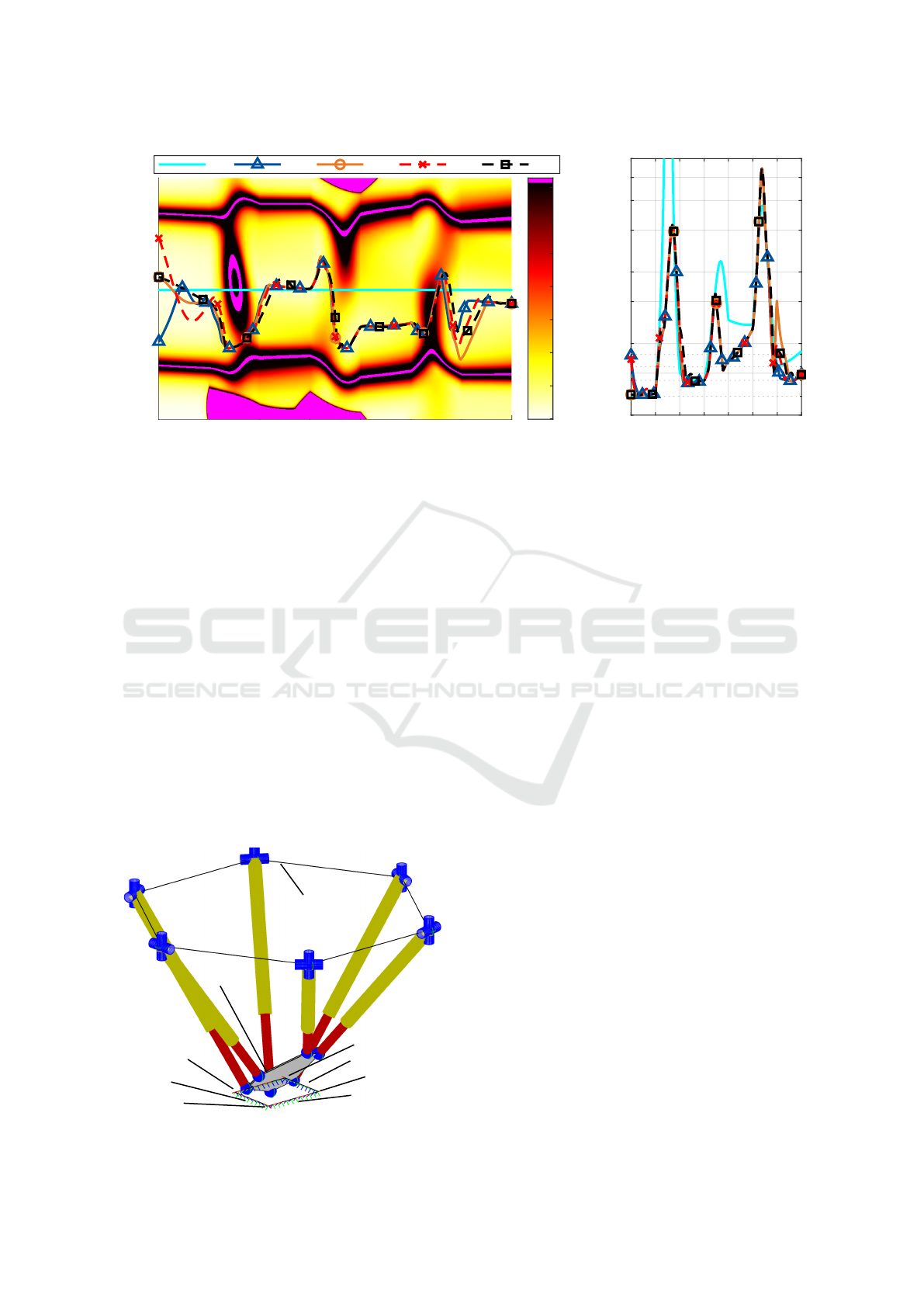
Figure 5: (a) Performance map of the condition number over the trajectory progress and all possibilities for the redundant

coordinate. (b) Distribution of the condition number over the trajectory for different settings.

q. The extent of oscillation and the settling time is

inﬂuenced by the selected rather low joint velocity

limits (see Table 1). This shows the feasibility of the

proposed nullspace scheme in full joint coordinates to

be able to leave a type-II singularity. The gain values

above are not directly comparable to the ones of sec-

tion 6.1.1, since there the compensation of the term

k(q

q) of (26) is attempted. The values in section 6.1.1

are divided by k

q,x

x) = ||

−1

||, which presents a

rough estimate. The determination of the exact rela-

tion is subject of ongoing work. Also, a general rule

to determine the controller gains has to be found.

6.2 Trajectory with Singularity

Avoidance

The previous evaluation of section 6.1 shows the gen-

eral property of the task coordinate’s nullspace to al-

s=0, s=7

1≤s≤2

3≤s≤4

5≤s≤6

4≤s≤5

2≤s≤3

robot base

trajectory

moving

platform

Figure 6: Starting pose of the robot trajectory for ϕ

=0.

low moving the manipulator away from singularities

without an additional task motion. In a practical ap-

plication like milling a pointing task trajectory y

y(t)

with C

differentiability (or higher) is given. There-

fore a task trajectory

(t) according to (20) is active

in the motion generation scheme summarized in Fig-

ure 1. Since milling presents one of the major use

cases of hexapod parallel robots, an exemplary trajec-

tory of milling a 45

◦

bezel to a rectangular pocket is

used for evaluation, as visualized in Figure 6. The red,

green and blue axes around the rectangle represent the

x-, y- and z-axis of the end effector frame for ϕ

=0.

Due to the task symmetry, only the pointing direction

of the blue z-axes has to be aligned. The tilting angle

of 45

◦

poses high requirements on the robot and em-

phasizes the necessity of an appropriate spatial orien-

tation representation. The trajectory is put together by

rest-to-rest motions between eight poses y

as points

of support, summarized in Table 2 and correspond-

ing to s =0 to s= 7 in Figure 6. At each corner of the

250 mm×200 mm-rectangle a change of orientation is

necessary to adjust the 45

◦

angle for the next edge,

corresponding to 1≤s≤2, 3≤s≤4 and 5≤s≤6 in Fig-

ure 6. A normalized trajectory coordinate s instead of

the time t is used to represent progress along the path

in the ﬁgures of this section for the sake of simplic-

ity. Each rest-to-rest motion is assigned a range of one

in s. However, the trajectory is generated by a trape-

zoidal acceleration proﬁle (C

time-differentiable S-

curve) with ˙r

max

=50 mms

−1

max

=10

◦

/s, a discrete

sample time of 1 ms and acceleration and jerk times

of 10 ms. The duration of the trajectory is 63.1 s.

The global distribution of the condition number

h(q

q,x

x) = cond(J

) is shown as a performance map in

ICINCO 2021 - 18th International Conference on Informatics in Control, Automation and Robotics

346

Figure 5 for the complete trajectory, represented by

1062 samples of the path coordinate s on the horizon-

tal axis. The vertical axis is chosen as the redundant

coordinate ϕ

which was discretized in 361 samples in

the range of ±180

◦

. The condition number is coded

by the color of the map. High condition numbers

h > 400 are saturated in the color code to dark red.

Singularities, which are deﬁned as condition numbers

h > 10

, and areas of joint limit violation are marked

with magenta. Creating the colored performance map

in this resolution requires 383 thousand evaluations

of the inverse kinematics and the performance crite-

rion. With this map a global optimization of the coor-

dinate ϕ

(s) can be performed, which corresponds to

the methods of the state of the art.

Using a local optimization on the contrary does

not require the expensive computation of the perfor-

mance map. The nullspace motion of the redundant

coordinate ϕ

is performed again by the nullspace

controller scheme of section 5. Different settings for

the nullspace controller are chosen for illustration and

the resulting nullspace motion is shown as different

lines in the performance map in Figure 5 a and as the

evolution of the condition number over the progress

of the trajectory in Figure 5 b. The settings are listed

in Table 3. Using different starting values and settings

emphasizes the robustness of the approach.

It has to be mentioned that the effects of the

nullspace gains are limited by the velocity and accel-

eration limits of the joints (see Table 1). Therefore

mainly in the last part of the trajectory a difference

between the settings becomes visible. The overall

behavior of avoiding areas of singularity is achieved

with all settings. The reference is a constant rotation

of the platform with ϕ

=30

◦

(cyan line in Figure 5).

This presents a good solution at the beginning, but

leads to a singularity during change of orientation at

the second corner for 1≤ s ≤ 2.

The ﬁrst nullspace setting (set 1) in Figure 5 cor-

responds to the ﬁrst setting in section 6.1.2. The other

settings each have different gains. All nullspace set-

tings produce a motion that avoids the ﬁrst area of

singularity at s ≈1.5. Also a second area of high, but

non-singular condition numbers at s ≈3.7 is avoided.

A third area of high condition numbers at s ≈5.4 can

not be avoided, since the shape of the performance

map leads to a dead end at the previous section of low

condition numbers at s >5. Here the disadvantage of

the local optimization becomes apparent and a global

optimization or a component of looking ahead (for

higher s) would outperform the proposed approach.

The qualitative effect of the decreasing gains and in-

creasing damping over the settings numbers can be

seen at parts of the trajectory where a reconﬁgura-

tion of the platform orientation is performed, e.g. at

s≈ 2.1 and s ≈5.9. For lower gains the optimal plat-

form rotation is achieved later (in the sense of time t

and therefore also of trajectory progress s).

6.3 Evaluation of Computation Time

The number of function evaluations required for the

determination of the gradients of performance objec-

tives obviously inﬂuences the computation time. The

inverse kinematics algorithms on position and trajec-

tory level were implemented in MATLAB as compiled

stand-alone functions (using the MATLAB code gen-

erator and mex ﬁles). This combines fast iterations

and efﬁcient debugging with the MATLAB graphical

user interface on the one hand and fast runtime of

C++ code on the other hand. The computation time

was evaluated on a standard desktop computer (Intel

Core i5-7500 CPU, 3.40 GHz, Linux operating sys-

tem, generic kernel, no real-time). The hardware per-

formance corresponds to typical PC-based robot con-

trollers. Measured computation times should be re-

garded relative to each other and in their order of mag-

nitude and may differ on other computing hardware.

Executing the position-level IK in the evaluation

of section 6.1 requires 394 steps with the Newton-

Raphson algorithm to compute an optimal pose which

takes a mean computation time of 226 ms (n=50,

σ=3.96 ms). The mean time per iteration is 0.57 ms

(σ=0.01 ms). This corresponds to the blue lines in

Figure 3. 555 iterations are necessary in section 6.1.2

with a similar mean time per iteration of 0.56 ms

(n=50, σ=0.01 ms, blue lines in Figure 4).

If a variation in all joint coordinates is com-

puted separately according to section 4.2.1, one it-

eration takes 1.78 ms (n=50, σ=0.04 ms). Despite

this method being not applicable to the case of sec-

tion 6.1, this shows the signiﬁcance of using the gra-

dient computation by the redundant coordinate’s dif-

ference quotient from section 4.2.2.

The computation of the null space motion in the

actuation space according to section 4.2.3 (and 6.1.1)

instead of the full joint space of section 4.2.2 (and

6.1.2) does not improve the computation time of the

trajectory IK as expected in the current implementa-

tion. A simulated time of 10 s and therefore 10,000

samples were computed to obtain the black and or-

ange lines in Figures 3 and 4. Timing evaluation

was performed with n=50 repetitions. In the actuated

joint space (Figure 3) the computation time was 9.3 s

(σ=52 ms, orange line, 0.93 ms per sample) and 9.7 s

(σ=243 ms, black line). In the full joint space (Fig-

ure 4) the computation times were 9.1 s (σ=147 ms,

orange line) and 9.2 s (σ=15 ms, black line). Using

Singularity Avoidance of Task-redundant Robots in Pointing Tasks: On Nullspace Projection and Cardan Angles as Orientation Coordinates

347

the MATLAB proﬁler on the non-compiled function

reveals that computing N

of section 4.2.2 only takes

about 3.5 % of the total time and N

of section 4.2.3

only takes about 0.6 % of the total time. Performing

the 6×6 inverse necessary for the latter approach only

takes 0.15 %. The term N

is also used for a nullspace

motion upon joint position limit violation and is com-

puted in all cases. This explains the higher compu-

tation times in the latter cases. Due to the small dif-

ferences between the computation times the full co-

ordinate space (section 4.2.2) should always be used

within the current implementation of the algorithm.

The effort for computing the nullspace motion in

general becomes visible when comparing the non-

redundant case in section 6.2 (cyan line in Figure 5) to

the redundant cases (other lines). The non-redundant

trajectory takes 12.7 s (n=10, σ=23 ms, 0.20 ms per

sample) while the redundant case takes 54.7 s (n=10,

σ=139 ms, 0.87 ms per sample).

In summary it can be stated that despite the higher

computational effort for the nullspace motion algo-

rithms already the current implementation can be used

as an online controller, since the runtime stays be-

low 1 ms, which is the typical control loop sample

time for such robots. The MATLAB functions can

be directly used as blocks in SIMULINK which can

be deployed with the EtherLab toolchain (using stan-

dard Ethernet hardware of a desktop computer with

Linux realtime kernel as target and the EtherCAT bus

as sensor/actuator interface). Runtime may further be

improved by disabling computations with little effect

and by using functions speciﬁc to the robot instead of

the currently used general approach without limiting

assumptions.

7 CONCLUSIONS AND

OUTLOOK

A simpliﬁed computation of the gradients of perfor-

mance criteria of robot manipulators is presented,

which exploits the properties of task redundancy of

degree one. This presents an extension to the appli-

cation of redundancy resolution frameworks for serial

and parallel robot manipulators. The performance cri-

teria have to be evaluated under real-time conditions

to allow their online optimization. Therefore, deploy-

ment of more sophisticated performance criteria will

be possible by reducing the number of function eval-

uations necessary for gradient calculation.

With the presented nullspace formulation avoid-

ing singularities for parallel robots is possible by per-

forming the calculations in the full joint space. Using

this more complex model allows to deﬁne a fallback

controller for exiting a singularity of type II. This can

be used if tracking a trajectory fails due to external

disturbance or in case of manually guiding a parallel

robot platform in teaching mode. In ofﬂine trajectory

planning such as for machining tasks the method can

be used to locally optimize path segments combined

with global optimization of the whole path similar to

Figure 5 of the paper.

Compared to the authors’ earlier work, the redun-

dancy resolution schemes of (Kotlarski et al., 2010)

are extended for an efﬁcient continuous adaption of a

redundant degree of freedom instead of the previously

favored discrete optimization. The need for computa-

tionally expensive global optimization decreases. The

theoretical contribution (Schappler et al., 2019) re-

garding kinematic modeling is brought one step closer

towards an application.

Future work comprises ﬁnding rules for setting

gain parameters of the nullspace scheme, ﬁnding the

analytic relation (26) between nullspace projectors of

parallel robot actuator space and full joint space, and

performing a stability analysis using control theory.

Table 1: Characteristic values of the parallel robot of Sec. 6.

Name Symbol Value Unit

base diameter d

1200 mm

platform diam. d

400 mm

(in Sec. 6.2) d

300 mm

joint pair distance d

100 mm

platform position r

, r

50, 30, 600 mm

platf. orientation ϕ

,ϕ

◦

,−30

◦

deg

act. j. stroke limits θ

i,min/max

600, 1200 mm

pass j. angle lim. — not set deg

act. j. velo. limits

i,max

2 ms

−1

pass j. velo. lim. — 45 deg/s

act. j. acc. limits

i,max

20 ms

−2

pass j. acc. lim. — 1146 deg/s

Table 2: Rest poses y

of the trajectory in Figures 5 and 6.

s r

mm mm mm deg deg

0 -50 40 700 45 0

1 200 40 700 45 0

2 200 40 700 0 -45

3 200 -160 700 0 -45

4 200 -160 700 -45 0

5 -50 -160 700 -45 0

6 -50 -160 700 0 45

7 -50 40 700 0 45

Table 3: Settings for the nullspace motion of the trajectory

in Figure 5 and Figure 6.

Param. ref. set 1 set 2 set 3 set 4

z,0

◦

−30

◦

— 0.03 0.1 0.25 0.5

— 0.05 0.01 0.005 0.0025

— 0.01 0.002 0.001 0.0005

ICINCO 2021 - 18th International Conference on Informatics in Control, Automation and Robotics

348

ACKNOWLEDGEMENTS

The authors acknowledge the support by the Deutsche

Forschungsgemeinschaft (DFG) under grant number

341489206. MATLAB Code to reproduce the results

is available at GitHub under free license at https://

github.com/SchapplM/robotics-paper_icinco2021.

REFERENCES

Agarwal, A., Nasa, C., and Bandyopadhyay, S. (2016). Dy-

namic singularity avoidance for parallel manipulators

using a task-priority based control scheme. Mecha-

nism and Machine Theory, 96:107–126.

Chiaverini, S., Oriolo, G., and Walker, I. D. (2008). Kine-

matically redundant manipulators. In Springer Hand-

book of Robotics, pages 245–268. Springer.

Corinaldi, D., Angeles, J., and Callegari, M. (2016). Pos-

ture optimization of a functionally redundant parallel

robot. In Advances in Robot Kinematics 2016, pages

101–108. Springer.

De Luca, A., Oriolo, G., and Siciliano, B. (1992). Robot

redundancy resolution at the acceleration level. Labo-

ratory Robotics and Automation, 4:97–97.

Gao, Y., Chen, K., Gao, H., Xiao, P., and Wang, L. (2019).

Small-angle perturbation method for moving platform

orientation to avoid singularity of asymmetrical 3-

RRR planner parallel manipulator. Journal of The

Brazilian Society of Mechanical Sciences and Engi-

neering, 41:1–18.

Gosselin, C. and Schreiber, L.-T. (2016). Kinematically

redundant spatial parallel mechanisms for singularity

avoidance and large orientational workspace. IEEE

Transactions on Robotics, 32(2):286–300.

Gosselin, C. and Schreiber, L.-T. (2018). Redundancy in

Parallel Mechanisms: A Review. Applied Mechanics

Reviews, 70(1).

Guo, Y., Dong, H., and Ke, Y. (2015). Stiffness-oriented

posture optimization in robotic machining applica-

tions. Robotics and Computer-Integrated Manufac-

turing, 27(2):367–376.

Huo, L. and Baron, L. (2008). The joint-limits and singu-

larity avoidance in robotic welding. Industrial Robot:

An International Journal, 35(5):456–464.

Kotlarski, J., Do Thanh, T., Heimann, B., and Ortmaier,

T. (2010). Optimization strategies for additional ac-

tuators of kinematically redundant parallel kinematic

machines. In 2010 IEEE International Conference on

Robotics and Automation (ICRA), pages 656–661.

Žlajpah, L. (2017). On orientation control of functional

redundant robots. In 2017 IEEE International Con-

ference on Robotics and Automation (ICRA), pages

2475–2482.

Léger, J. and Angeles, J. (2016). Off-line programming

of six-axis robots for optimum ﬁve-dimensional tasks.

Mechanism and Machine Theory, 100:155–169.

Lillo, P. D., Chiaverini, S., and Antonelli, G. (2019). Han-

dling robot constraints within a set-based multi-task

priority inverse kinematics framework. In 2019 IEEE

International Conference on Robotics and Automation

(ICRA), pages 7477–7483.

Luces, M., Mills, J. K., and Benhabib, B. (2017). A review

of redundant parallel kinematic mechanisms. Journal

of Intelligent & Robotic Systems, 86:175–198.

Merlet, J.-P. (2006). Jacobian, manipulability, condition

number, and accuracy of parallel robots. Journal of

Mechanical Design, 128(1):199–206.

Merlet, J.-P., Perng, M.-W., and Daney, D. (2000). Optimal

trajectory planning of a 5-axis machine-tool based on

a 6-axis parallel manipulator. In Advances in Robot

Kinematics, pages 315–322. Springer.

Mousavi, S., Gagnol, V., Bouzgarrou, B. C., and

Ray, P. (2018). Stability optimization in robotic

milling through the control of functional redundan-

cies. Robotics and Computer-Integrated Manufactur-

ing, 50:181–192.

Nakamura, Y., Hanafusa, H., and Yoshikawa, T. (1987).

Task-priority based redundancy control of robot ma-

nipulators. The International Journal of Robotics Re-

search, 6(2):3–15.

Oen, K.-T. and Wang, L.-C. T. (2007). Optimal dynamic

trajectory planning for linearly actuated platform type

parallel manipulators having task space redundant de-

gree of freedom. Mechanism and Machine Theory,

42(6):727–750.

Ozgoren, M. K. (2013). Optimal inverse kinematic solu-

tions for redundant manipulators by using analytical

methods to minimize position and velocity measures.

Journal of Mechanisms and Robotics, 5(3).

Reiter, A., Müller, A., and Gattringer, H. (2018). On higher

order inverse kinematics methods in time-optimal tra-

jectory planning for kinematically redundant manipu-

lators. IEEE Transactions on Industrial Informatics,

14(4):1681–1690.

Santos, J. C. and da Silva, M. M. (2017). Redundancy res-

olution of kinematically redundant parallel manipula-

tors via differential dynamic programing. Journal of

Mechanisms and Robotics, 9(4).

Schappler, M., Tappe, S., and Ortmaier, T. (2019).

Modeling parallel robot kinematics for 3T2R and

3T3R tasks using reciprocal sets of Euler angles.

MDPI Robotics, 8(3). Open access journal. Online:

https://doi.org/10.3390/robotics8030068.

Shaw, D. and Chen, Y.-S. (2001). Cutting path generation

of the stewart-platform-based milling machine using

an end-mill. International Journal of Production Re-

search, 39(7):1367–1383.

Smirnov, V., Plyusnin, V., and Mirzaeva, G. (2013). Energy

efﬁcient trajectories of industrial machine tools with

parallel kinematics. In 2013 IEEE International Con-

ference on Industrial Technology (ICIT), pages 1267–

1272.

Zhu, W., Qu, W., Cao, L., Yang, D., and Ke, Y. (2013).

An off-line programming system for robotic drilling

in aerospace manufacturing. The International Jour-

nal of Advanced Manufacturing Technology, 68(9-

12):2535–2545.

Singularity Avoidance of Task-redundant Robots in Pointing Tasks: On Nullspace Projection and Cardan Angles as Orientation Coordinates

349