A Reference Process for Judging Reliability of Classiﬁcation Results in

Predictive Analytics

Simon Staudinger

, Christoph G. Schuetz

and Michael Schreﬂ

Institute of Business Informatics, Data and Knowledge Engineering, Johannes Kepler University Linz, Austria

Keywords:

Business Intelligence, Business Analytics, Decision Support Systems, Data Mining, CRISP-DM.

Abstract:

Organizations employ data mining to discover patterns in historic data. The models that are learned from

the data allow analysts to make predictions about future events of interest. Different global measures, e.g.,

accuracy, sensitivity, and speciﬁcity, are employed to evaluate a predictive model. In order to properly assess

the reliability of an individual prediction for a speciﬁc input case, global measures may not sufﬁce. In this

paper, we propose a reference process for the development of predictive analytics applications that allow

analysts to better judge the reliability of individual classiﬁcation results. The proposed reference process is

aligned with the CRISP-DM stages and complements each stage with a number of tasks required for reliability

checking. We further explain two generic approaches that assist analysts with the assessment of reliability of

individual predictions, namely perturbation and local quality measures.

1 INTRODUCTION

Organizations employ data mining to discover pat-

terns in historic data in order to learn predictive mod-

els. The CRoss-Industry Standard Process for Data

Mining (CRISP-DM) (Wirth and Hipp, 2000) serves

as guideline for the proper application of data mining,

aligning data analysis with the organization’s busi-

ness goals. The CRISP-DM comprises six stages:

(i) business understanding, (ii) data understanding,

(iii) data preparation, (iv) modeling, (v) evaluation,

and (vi) deployment. The CRISP-DM is widely em-

ployed in data-analysis projects in various domains

(Caetano et al., 2014; Moro et al., 2011; da Rocha

and de Sousa Junior, 2010).

The predictive models that are learned from data

allow decision-makers to make predictions about fu-

ture events of interest and act accordingly. The pre-

dictions of learned models may be more or less accu-

rate, raising the question about the reliability of indi-

vidual predictions. Consider, for example, a classiﬁ-

cation model that allows a bank employee to decide

whether a speciﬁc client will default on a requested

loan in the future. If similar cases from the past can-

not be clearly associated with a speciﬁc outcome, or

https://orcid.org/0000-0002-8045-2239

https://orcid.org/0000-0002-0955-8647

https://orcid.org/0000-0003-1741-0252

similar cases have not been present in the input data,

the prediction will not be very reliable. Nevertheless,

the model will come up with a prediction, but it is

up to the analyst to judge on the reliability of that

prediction. If actions are based on unreliable predic-

tions, this could lead to potentially costly failures and

missed business opportunities.

When it comes down to judging the reliability

of an individual prediction, the accuracy and simi-

lar quality measures of the entire model are often the

only guidance available. The accuracy is a summary

of the overall performance of the model, which is not

enough to make a robust statement about the relia-

bility of an individual prediction for a speciﬁc input

case. For example, a model’s training data points may

not be evenly distributed in the feature space. A new

data point located in a densely populated part of the

feature space may obtain a more reliable prediction

than a new data point in a sparsely populated part.

The overall accuracy of the model would be the same

for both predictions. Other works (Moroney, 2000;

Capra et al., 2006; Reimer et al., 2020; Vriesmann

et al., 2015) have shown that it can be fruitful to in-

vestigate models and collect model metrics not only

on a global level but also in the local area of interest

of the data. Calculating local quality measures, e.g.,

the local accuracy of a model for a speciﬁc prediction

case, conveys a better impression of the reliability of

an individual prediction than using the global measure

124

Staudinger, S., Schuetz, C. and Schreﬂ, M.

A Reference Process for Judging Reliability of Classiﬁcation Results in Predictive Analytics.

DOI: 10.5220/0010620501240134

In Proceedings of the 10th International Conference on Data Science, Technology and Applications (DATA 2021), pages 124-134

ISBN: 978-989-758-521-0

for the model as a whole. Furthermore, taking inspi-

ration from the ﬁeld of numerical analysis, where the

condition number describes the magnitude of change

of a function’s output in the face of small changes of

the function’s input (Cheney and Kincaid, 2012), we

propose to employ perturbation of input data for in-

dividual prediction cases in order to better judge on

the reliability of a prediction: If small changes in the

input data of a speciﬁc prediction case lead to a com-

pletely different prediction, the reliability of that pre-

diction is questionable. For example, in the context of

the prediction of a loan default by a prospective cus-

tomer, if a small change in the monthly income leads

to an opposite prediction for loan default, the predic-

tion may not be very reliable since a small change in

monthly income is very likely to happen.

In this paper, we propose a reference process

based on CRISP-DM for building predictive analytics

applications that allow analysts to judge the reliability

of individual classiﬁcation results. We illustrate that

generic reference process over a real-world data set

from a telemarketing campaign of a Portuguese bank

(Moro et al., 2014). We propose that in order to bet-

ter judge the reliability of individual predictions, an

analyst must consider the actual input data, the data

used for training the predictive model, and the spe-

ciﬁc procedures regarding collection and preparation

of the data. The proposed reference process deﬁnes

tasks along the entire CRISP-DM life cycle. During

the business understanding stage, the reference pro-

cess requires developers of predictive analytics appli-

cations to choose between different approaches for re-

liability checking. The data understanding and data

preparation stages then require the gathering of fur-

ther information about the available data and poten-

tial reliability problems arising from data collection.

The information about the available data subsequently

serves to select and conﬁgure the approaches for reli-

ability checking, which are then evaluated regarding

suitability for the given analytics problem. When the

model is deployed, the additionally deﬁned modules

for reliability checking can be used by the analyst to

better judge the reliability of an individual prediction

and to better decide how to properly act on the predic-

tion. Given an already trained black-box or white-box

model, the tasks assisting in judging the reliability re-

sults can still be added, opening up the possibility to

use the reference process for prediction models which

are already in use.

We follow a design science approach (Hevner

The employed data set is available on the UCI Ma-

chine Learning Repository via the link https://archive.ics.

uci.edu/ml/datasets/bank+marketing (accessed: 1 March

2021).

et al., 2004). The goal of design science research is

the development of design artifacts that solve a prac-

tical problem. A design artifact can be a model but

also a method or software tool. The contributions of

this paper are two design artifacts: a generic reference

process and the use of perturbation options within the

reference process.

The remainder of this paper is organized as fol-

lows. In Section 2, we review related work. In Sec-

tion 3, we give an overview of the proposed reference

process. In Section 4, we describe the tasks related

to data collection and data preprocessing as well as

guidelines to adapt a speciﬁc classiﬁcation problem.

In Section 5, we focus on tasks related to modeling

and evaluation. In Section 6, we discuss deployment

of the reference process, illustrated on the use case.

In Section 7, we conclude the paper with a summary

and an outlook on future work.

2 RELATED WORK

In various domains, dynamic classiﬁer selection

(DCS) is used in multiple classiﬁer systems to ﬁnd the

best classiﬁer for a given classiﬁcation problem and a

given classiﬁcation case (Cruz et al., 2018). In com-

parison to majority voting, where the ﬁnal outcome is

the class predicted by the most classiﬁers, DCS aims

to ﬁnd the best-ﬁtting classiﬁer for the individual case

and use the prediction of this classiﬁer as the ﬁnal

outcome. Different approaches to ﬁnd the best classi-

ﬁers, including the use of local regions within the fea-

ture space were already examined (Cruz et al., 2018;

Didaci et al., 2005; Vriesmann et al., 2015).

The problem of judging reliability of predictions

is related to metamorphic software testing. Meta-

morphic testing is concerned with the oracle problem

in software testing. This problem occurs in systems

where the correct behavior cannot be distinguished

from the incorrect behavior due to missing formal

speciﬁcations or assertions. For more information on

metamorphic testing we refer to other works (Barr

et al., 2015; Chen et al., 2018; Segura et al., 2016).

The central points of interest in this area are the meta-

morphic relations, which describe the differences be-

tween input and output of a software system. The out-

put is called a follow-up test case and can again be

used as input for a metamorphic relation, creating a

possibly inﬁnite amount of potential test cases. If the

real outcome of the software system is different than

the expected one there is likely an error within this

system. An example of a metamorphic relation is the

case of two search queries, where the second query

restricts the ﬁrst query. If during metamorphic testing

A Reference Process for Judging Reliability of Classiﬁcation Results in Predictive Analytics

125

the result of the second query is not a subset of the

ﬁrst query, the query implementation is faulty. The

difﬁcult and challenging part in metamorphic testing

is to ﬁnd metamorphic relations suitable for the exist-

ing software models to be tested. Metamorphic test-

ing has also been used in the domain of predictive an-

alytics. There are multiple works which examine the

use of metamorphic relations to ensure the soundness

of machine-learning classiﬁers (Xie et al., 2011; Saha

and Kanewala, 2019; Moreira et al., 2020).

The main contribution of the paper is the refer-

ence process for judging the reliability of predictive

analytics results. To the best of our knowledge, no

other such process has been proposed yet. The pro-

posed reference process contains tasks that include

aspects of related work. The tasks adapt the follow-

ing ideas from related work. First, while DCS focuses

on the selection of the best classiﬁer through the use

of local measures, DCS does not consider using lo-

cal measures to evaluate the reliability of individual

predictions made by the same classiﬁer. We use the

local-region approach within our reference process to

ﬁnd differences between global and local measures

for individual cases within the same classiﬁer. Sec-

ond, metamorphic testing uses slightly different input

cases in combination with a metamorphic relation to

ensure the correctness of a system. We employ the ap-

proach of input-case perturbation to test if small input

variations inﬂuence the prediction.

3 REFERENCE PROCESS:

OVERVIEW

We propose a reference process for judging reliabil-

ity of classiﬁcation results, which we organize along

the CRISP-DM stages (Figure 1). In order to arrive at

predictive analytics applications that facilitate judg-

ment of reliability of individual predictions, at each

stage of the CRISP-DM, additional tasks have to be

considered by developers and analysts. During busi-

ness understanding, appropriate approaches for relia-

bility checking must be selected under consideration

of the business and data mining goals. An example of

such an approach is to use perturbation of test cases

to ﬁnd features in the data that are especially sensi-

tive regarding the prediction. Data understanding in

CRISP-DM is concerned with collection and review

of the available data. Judging reliability at later stages

requires the use of metadata and, therefore, the meta-

data need to be collected and documented during the

data-understanding stage. Gathered metadata may in-

clude, for example, the scale of the feature, the preci-

sion of the measured feature value, and existing data

restrictions, e.g., allowed feature ranges.

Raw data are typically not suitable as training

data. Hence, the data preparation stage typically ap-

plies a multitude of techniques to increase the data

quality and provide the data in a suitable format for

training. Applying data preparation techniques can

result in various reliability issues and, therefore, the

employed data preparation techniques should be doc-

umented. For example, issues may arise when han-

dling missing data or discretizing values.

In the modeling stage, two approaches for relia-

bility checking are considered: the perturbation of in-

put cases and the evaluation of local quality measures.

Using the information from the previous steps allows

the modeler to choose and conﬁgure these approaches

with regard to the actual analysis case. Input pertur-

bation aims to ﬁnd sensitive features and possible bor-

derline predictions. Local measures allow to compare

the global performance of the model with the perfor-

mance of the individual case. The conﬁguration of

these approaches is done for every data mining prob-

lem. Once deﬁned, these approaches can be used to

judge the reliability of different input cases once the

model has been deployed.

The parameters of the approaches for reliability

checking need to be ﬁtted to the data mining problems

and the individual use cases. A ﬁrst assessment of the

chosen parameters will be conducted during the eval-

uation stage. Example parameters include the range

of the perturbation or the distance for the calculation

of the local measures.

The last stage in the CRISP-DM is the deployment

of the trained model. New input data that are passed

to the model will receive a prediction. An analyst can

use the deﬁned and assessed approaches to judge the

reliability of the received prediction. If none of the

predeﬁned approaches is suitable, the approaches can

be adapted or new approaches can be deﬁned in order

to improve the quality of the judgment of the reliabil-

ity of a prediction.

We note that the presented reference process, al-

though illustrated and discussed on the example of

classiﬁcation, is not limited to the problem of clas-

siﬁcation but potentially also applicable for other pre-

diction problems. In the following, we present in

more detail the different tasks of the reference pro-

cess along the different stages of the CRISP-DM.

DATA 2021 - 10th International Conference on Data Science, Technology and Applications

126

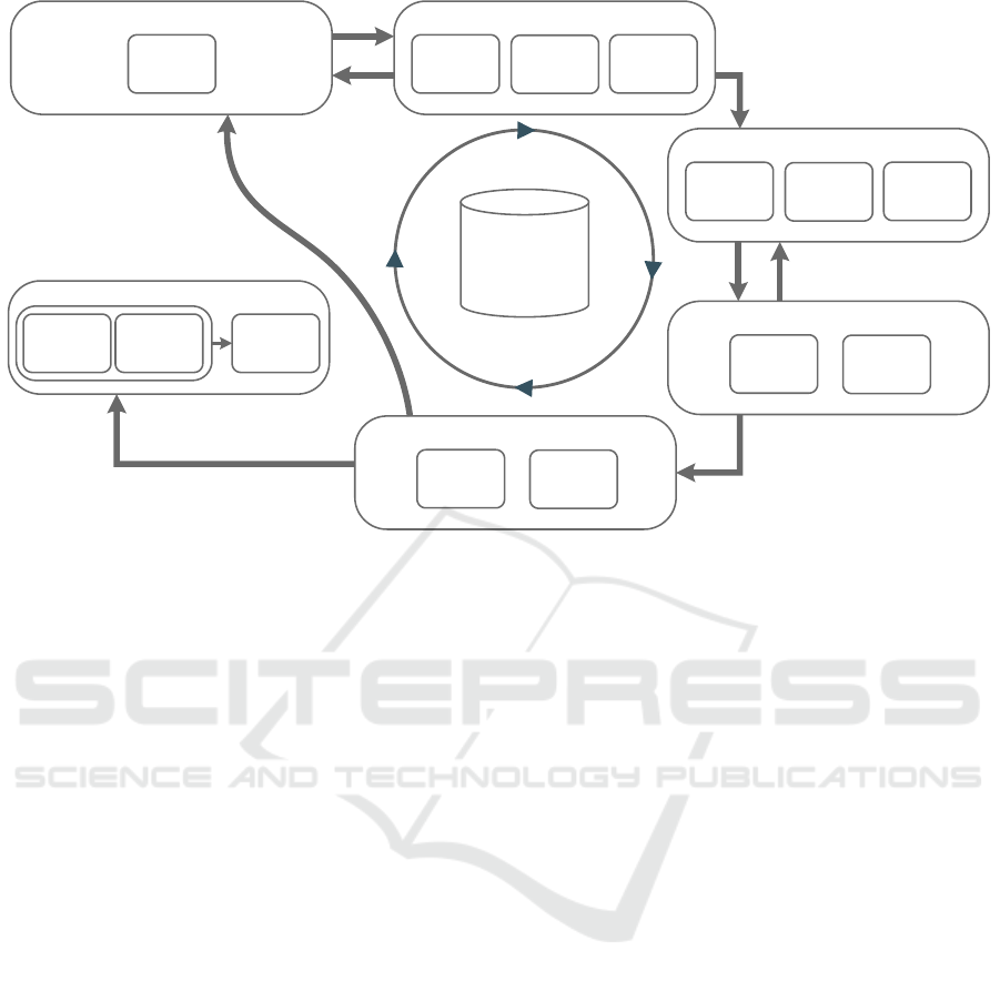
Data

Evaluation

Evaluation of

Local Quality

Measures

Evaluation of

Perturbation

Options

Business Understanding

Choice of

Reliability

Approaches

Data Preparation

Documentation

of Range of

Binned

Features

Documentation

of Handling of

Missing Values

Documentation

of Regression

Function

Metrics

Modeling

Definition and

Choice of Local

Quality

Measures

Definition and

Choice of

Perturbation

Options

Deployment

Reliability

Judgment

Measurement

of Local

Quality

Measures

Perturbation of

Classification

Case

Data Understanding

Determination

of Scale of

Features

Determination

of Volatility of

Features

Determination

of Data

Restrictions

Figure 1: Overview of the reference process for judging reliability of classiﬁcation results along the CRISP-DM stages.

4 BUSINESS UNDERSTANDING,

DATA UNDERSTANDING AND

DATA PREPARATION

Business understanding is concerned with the deﬁ-

nition of both business and data mining goals that

should be reached within the data mining process.

In addition to these goals, it must be decided in

which way the reliability of the predictions should

be assessed. Given different reliability-checking ap-

proaches, the ﬁt of each approach for the use case

must be considered, and whether it is possible to em-

ploy those approaches. For example, if local mea-

sures for each new case are desired there must be ac-

cess to the training data. If the organization is inter-

ested in ﬁnding sensitive input features, the perturba-

tion approach may be a good ﬁt in order to judge the

reliability of individual predictions. In this paper, we

describe two approaches, but future work will inves-

tigate other approaches, e.g., the use of genetic algo-

rithms to ﬁnd possible border cases.

There are different types of data that are of inter-

est for the analysis, e.g., structured data, streaming

data, images, and videos. During data collection and

extraction, inaccuracies may slip into the data, or it

might even be impossible to capture the exact value.

If we know the range of these inaccuracies, or at least

that a feature might be different compared to the real

value, we can use this information later when judg-

ing the reliability of a prediction. A prime example of

inaccuracy of the collected data is sensor imprecision

(Guo et al., 2006). Information about imprecision of

the collected data should be stated for every collection

method that is employed.

Data understanding and data preparation are nec-

essary stages before a data mining algorithm can be

used to train a predictive model. Every saved data

point has to be extracted from the real world. In this

paper, we focus on the case of structured data and

we provide guidelines that can be followed during the

data understanding and data preparation stages in or-

der to subsequently be able to judge the reliability of

a prediction based on the collected information about

the following characteristics of the data.

Level of Measurement. Each feature has a level of

measurement, which should be determined during the

data understanding. The level can either be nominal,

ordinal, or cardinal.

Volatility of Feature Values. Features may have

different degrees of volatility. For example, a feature

that states if a customer has already been contacted

can assume the values “yes” or “no”. If the month of

a phone call is documented, there is no inherent un-

certainty about the real-world month. In contrast, for

example, wind speed may quickly change. The mea-

sured wind speed may be different if measured a few

minutes earlier.

A Reference Process for Judging Reliability of Classiﬁcation Results in Predictive Analytics

127

Feature Value Restrictions. Restrictions regard-

ing feature values can either be formal or domain-

speciﬁc. An example of a formal restriction is the

age of a person, which cannot be negative. A possible

example of a domain-speciﬁc restriction could be that

a person under the age of 18 is not allowed to open a

long-term deposit. The valid age range starts with the

value 18.

Data Accuracy. Depending on how a feature value

is collected, different kinds of precision can be

stated. First, the accuracy may depend on whether

the values were rounded when gathering the data.

For example, a salary given in thousands is most

likely not the exact value but in reality is slightly

less or more. Therefore, it is important to document

the range of the rounded value. For example, the

interval [950, 1050] may describe a given value of

1000 further. If any kind of technical device is used

to collect the data, it should be stated how accurate

the collected values are compared to the real values.

This may be given either as an absolute value, e.g.,

the measured value is correct within the range ±

0.5, as a relative value, e.g., ± 1%, or as accurate to

a certain number of decimal places. If features are

ordinal or nominal, and other feature values would

ﬁt as well for an individual data point, this should be

documented as well.

After the data have been collected and the qual-

ity documented, the data preparation stage includes

different techniques to improve the data quality and

to transform the data in a format that can then be

used to train the model. Similar to data understand-

ing, the employed techniques may be the reason why

inaccuracies were included in the data. In order to

tackle data quality issues concerning accuracy, con-

sistency, incompleteness, noise, and interpretability,

values can be altered or estimated. A possible ex-

ample may be the rounding of values, e.g., a given

income can be rounded to hundreds. Furthermore,

dealing with missing values in the data is another po-

tential concern when assessing the reliability of a pre-

diction. Since these values are just estimates, the in-

formation carried by the values is less precise than the

actual values. In the following, we enumerate several

cases where reliability-related information should be

collected.

Binned Features. To reduce the number of differ-

ent data points, binning can be applied to raw data. As

with rounded values, the binned value is an estimate,

and its possible bin range should be documented.

Regression Functions. If a regression function is

used during data preparation in order to obtain the fea-

ture values, evaluation metrics of the regression func-

tion should be documented, e.g., the R

value.

Missing Values. Different approaches exist for

dealing with missing values. For example, the mean

value of all available feature values may substitute

for a missing value. Alternatively, the standard value,

a placeholder, or a more sophisticated completion

mode, e.g., Markov chains, can be used. The method

for completing missing values should be documented.

The list of data preparation techniques mentioned

here is not exhaustive. In any case, the performed data

preparation technique, when altering the data, should

be documented and that information can then be used

in the further phases of the reference process to judge

the reliability of the predictions.

5 MODELING AND EVALUATION

In this section, we discuss the deﬁnition and evalu-

ation of reliability-checking approaches. Depending

on the classiﬁcation problem, different approaches

and parameters may be useful, which have to be eval-

uated. The selected and evaluated approaches can

then be used by the business user to get an insight

into the reliability of a speciﬁc prediction. This pa-

per describes two approaches: the perturbation of test

cases and the use of local quality measures.

5.1 Perturbation

A perturbation option is a formal description of a

function that generates neighboring values of a fea-

ture from the case considered for prediction, slightly

different from the case’s feature value. The perturba-

tion approach was inspired by the ﬁeld of numerical

mathematics, where the condition number measures

the effect of a changed input to the output of a given

function (Cheney and Kincaid, 2012). Each pertur-

bation option is assigned to a feature and takes the

original value of the feature as input. Depending on

the perturbation option, there can be additional input

parameters, e.g., the precision of a sensor, which are

required to apply the perturbation option during de-

ployment. The perturbation options often rely on a

speciﬁc scale of the feature. Since a deﬁned perturba-

tion option may not only be useful for one feature, the

scale of the feature is added to the deﬁnition. Fur-

thermore, each perturbation option is assigned one

of three levels. These levels assist the analyst with

DATA 2021 - 10th International Conference on Data Science, Technology and Applications

128

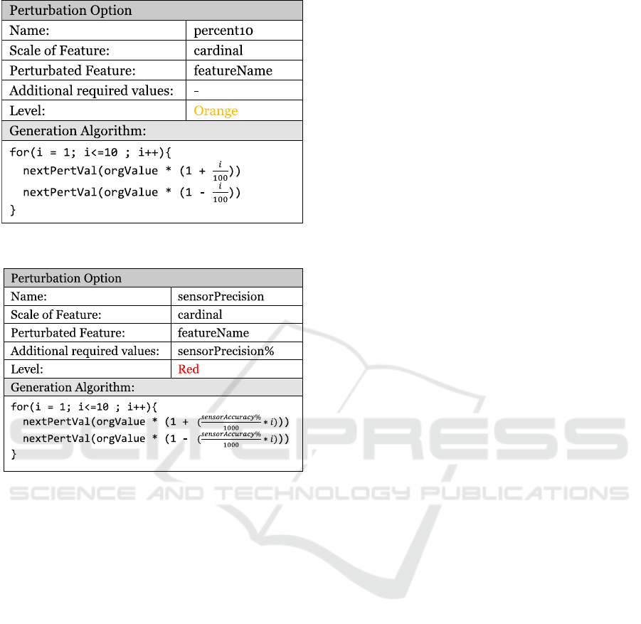
Figure 2: Option 10percent.

Figure 3: Option sensorPrecision.

judging the reliability of a prediction by indicating

which information from the data understanding and

data preparation stages led to the deﬁnition of the per-

turbed test case. The possible levels are red, orange,

and green. A red-level perturbation option states that

the prediction should not change while using values

generated with this perturbation option. An orange-

level perturbation option leading to a changed result

needs further examination since, the considered case

for prediction could be a border case to another classi-

ﬁcation label. A green-level perturbation option states

that the prediction is expected to change when per-

turbing the values, which means that the change does

not indicate a problem with the reliability of the actual

prediction.

Figure 2 and Figure 3 show example perturbation

options. The orgValue placeholder represents the

value from the original test case and nextPertVal

returns the perturbed value which is further used to

create the perturbed test case. The ﬁrst option (per-

cent10) describes a relative perturbation of a cardinal

value. The original value is increased/decreased rel-

atively to the considered case’s value, from ± 1% up

to ± 10%. Since an increase/decrease of a value can

lead to a changed prediction when reaching a border

case in the feature space, the level of the perturbation

option is orange, signifying that a changed prediction

can happen when perturbing the original case, which

requires the attention of the analyst. The second per-

turbation option (sensorPrecision) is a red-level op-

tion. The sensorPrecision option is intended to be

used for a value generated by a sensor. Every sensor

value is captured with a certain accuracy depending

on the device used for sensing. The real value lies

anywhere within the precision range. Since we do not

know the real value, the values in the precision range

should not change the prediction of a test case. The

red-level states that a changed prediction should not

happen for these values, because we do not know the

real-world value within this perturbation range. If the

prediction changes for a variation of the input value

that is within the sensor precision, the prediction is

not reliable.

A perturbed test case corresponds to the original

case for which we want to predict a value but with

one or more features swapped according to the value

supplied by the perturbation option. Each perturbed

test case is then passed to the model to obtain a pre-

diction. Predictions are then used to judge the relia-

bility of the original test case. For a combination of

different perturbation options, the highest level of the

options is assigned to the test case. Red is the highest

level, followed by orange and green.

In the previous section, we described the collec-

tion and preprocessing of the data as well as the ad-

ditional metadata that should be collected for judging

reliability. The additional information can be used to

deﬁne perturbation options based for a speciﬁc use

case. The perturbation options may be reused or

adapted for different features and classiﬁcation prob-

lems. A guideline for the deﬁnition and speciﬁcation

of different perturbation options depending on differ-

ent criteria follows.

Scale of Feature. Any feature for which the scale

is known can use one of the following kinds of per-

turbation options. Nominal features do not provide

any kind of order. Therefore, one option would be

to swap all available values. For ordinal features it is

also possible to swap all available features, but since

we have an order given it would be possible to use a

ﬁxed number of steps in one or both directions. Car-

dinal features can either be altered by relative or ab-

solute values. An example of a percent perturbation

option can be seen in Figure 2.

A Reference Process for Judging Reliability of Classiﬁcation Results in Predictive Analytics

129

Volatility. Knowing the volatility of a feature al-

lows for the deﬁnition of different perturbation op-

tions. If a feature is known to be volatile in the real

world it may be good to create perturbation options

for checking the values around the original feature

value. If a feature is known to be stable in the real

world, it is less likely that there are inaccuracies in

the values.

Accuracy. The accuracy of the data can also be a

good hint for the creation of perturbation options for

a feature. The known accuracy range or a known de-

viation can be used by a perturbation option to create

values within an interval. The prediction is expected

to stay the same for all values within the interval.

The perturbation options dealing with this informa-

tion should be assigned a red level. If values are esti-

mated, e.g., using a default value for a missing value,

binned feature values, or regression function values,

it can also be useful to create perturbation options re-

turning neighboring feature values. The creation of

accuracy-related perturbation options can be done for

any kind of known imprecision within the feature val-

ues.

Restrictions. If there are any value restrictions

identiﬁed during the analysis of the data, these

restrictions can be used to reduce the number of

perturbed values. If a perturbation option would

return a value violating the restrictions, the perturbed

value can be discarded and is not used for further

analysis.

The larger the number of perturbed cases that

are created and for which a prediction is obtained,

the more meaningful the judgment of the reliability

of the original case will become. In the best case,

all possible perturbed test cases are created and pre-

dicted. Since it is not practical and sometimes not

even possible to create all potential perturbed cases

due to restrictions regarding execution time or num-

ber of cases, it is necessary to use a speciﬁed oper-

ation mode. Each of the following operation modes

creates perturbed cases until either all possible com-

binations are provided, or the speciﬁed execution time

is reached. In the following, we describe three differ-

ent operation modes for perturbation.

Operation Mode: Full. The ﬁrst operation mode

computes all possible combinations of perturbed

cases. The operation mode starts by iterating through

all the available perturbation options. There is no pre-

ferred order in which the perturbation options should

age

job

marital

default

technician

single

technician

single

technician

single

technician

single

technician

married

technician

divorced

technician

single

yes

technician

married

technician

divorced

…

Perturbation

Option 1

Perturbation

Option 2

single

married

divorced

Perturbation

Option 3

yes

Figure 4: Operation mode: full.

be used. Each value of the selected perturbation op-

tion is inserted in the original case for the speciﬁed

feature and the perturbed case is used as input for the

model to obtain a prediction. In case that multiple per-

turbation options on different features are used, com-

binations of perturbation options are created. Combi-

nation of options continues until all possible combi-

nations have been created and prediction values have

been obtained. An example can be seen in Figure 4.

The ﬁrst line shows the original test case. Given the

values from the perturbation options shown at the bot-

tom of Figure 4, the displayed perturbed test cases are

generated. Each value from the perturbation options

is inserted into the original test case. All possible

combinations of values are created.

Operation Mode: Prioritized. The second pertur-

bation mode is similar to the ﬁrst operation mode. If

there is no time restriction in place, both will come

up with the same perturbed cases. Nevertheless, the

order in which the cases are created is changed. This

mode allows the user to explicitly mark perturbation

options as more important than others. For example,

if an analyst knows that the features income and age

are very important in the analysis, it can be stated that

perturbation options applied on these features should

be used with priority over other perturbation options.

Each value of the perturbation option is inserted into

the original case for a speciﬁed feature and is used

to predict a result. Afterwards, all the combinations

with the prioritized perturbation options are created.

DATA 2021 - 10th International Conference on Data Science, Technology and Applications

130

age

job

marital

default

technician

single

technician

single

technician

single

technician

single

technician

single

yes

technician

single

yes

technician

single

yes

technician

single

yes

Figure 5: Operation mode: selected.

Following this, all the remaining perturbations will be

created, predicted, and can be used for judging the re-

liability.

Operation Mode: Selected. The third mode only

takes a deﬁned number of perturbation options for the

generation of the perturbed cases. Instead of generat-

ing all available perturbed cases, only combinations

of predeﬁned perturbed cases are generated and

predicted, leading to a reduced subset of the cases

with respect to the cases retrieved using Full and

Prioritized mode. Columns with assured values or

values that are uninteresting from a business perspec-

tive can be skipped for the beneﬁt of faster execution

time. There is no predeﬁned order in which selected

perturbation options are used. Figure 5 shows an

example for the resulting perturbed test cases when

only Perturbation Option 1 and Perturbation Option 2

from Figure 4 are used during the selected mode.

After creating the perturbation options based on

the gathered information these perturbation options

can be assessed if they are ﬁt for the classiﬁcation

problem. Different perturbation options use param-

eters such as the percent value in the perturbation op-

tion shown in Figure 2. These parameters may be un-

suitable for a speciﬁc feature or classiﬁcation prob-

lem. During the evaluation stage of the CRISP-DM,

it can be tested if the chosen perturbation options and

parameters are suitable. For example, changing the

percent values/absolute values when they are not suit-

able for the given test case. If broader or narrower

perturbation options are needed to receive reasonable

results while applying the perturbation options on test

cases, they can be created or adapted before the model

is deployed.

5.2 Local Measures

A different approach for gathering information about

the reliability of a prediction is the use of local mea-

sures. If there is access to the training data, various

local measures can give an insight into the reliability

of the prediction. An example of a local measure is

the local accuracy (Woods et al., 1997). The over-

all accuracy provides the number of correct predic-

tions compared to the number of wrong predictions

for the whole model whereas the local accuracy dif-

ferentiates between different areas within the model.

It can be useful to know if the accuracy changes in

different areas of the feature space. Consider an over-

all prediction accuracy of 85% for the entire model.

There may be different subspaces that have a differ-

ent local accuracy compared to the overall accuracy.

Therefore, we can evaluate the local accuracy using

either a predeﬁned number of training set neighbors

or all training set neighbors in a predeﬁned distance

around the new classiﬁcation case. The surrounding

neighbors of a test case are selected using a distance

function, which calculates every distance between the

new test case and the given training set cases using,

for example, Euclidean distance. This can give an

insight into how well the algorithm performs in the

input data space around the new classiﬁcation case,

compared to the overall accuracy of the whole model.

A prediction for a case where the local accuracy of

the model is much lower than the overall accuracy of

the model as a whole should be mistrusted. For exam-

ple, a new case in a feature space with only 60% local

accuracy compared to 85% for the whole model has

a signiﬁcantly worse performance than stated by the

global measure. To receive a meaningful judgment,

there needs to be a reasonable number of training set

neighbors affected by the calculation. If this is not the

case the number of training set cases affected by the

local accuracy should be increased, or the local accu-

racy should not be considered when judging the relia-

bility of the prediction until the number is adapted.

Similar to the local accuracy, there is the local

class ratio. If we have access to the training data of

the model, we can use this information to provide an

insight into the ratio of the same training set neigh-

bor labels as our prediction compared to the different

neighboring labels in the training set. We are inter-

ested in how many of these neighbors have the same

label as our prediction. Accuracy measures just the

overall correctness of all test cases. Since we are in-

terested in a speciﬁc predicted label, the local class ra-

tio states the amount of training set neighbors with the

same real label within a predeﬁned number of neigh-

bors or all neighbors in a predeﬁned distance around

the new classiﬁcation case. To receive a meaningful

judgment, there needs to be a reasonable number of

neighbors affected by the calculation. If this is not the

case the number of training set cases affected by the

A Reference Process for Judging Reliability of Classiﬁcation Results in Predictive Analytics

131

local class ratio should be increased, or the local class

ratio should not be considered while judging the reli-

ability of the prediction until the number of neighbors

in the training set is adapted to a suitable number.

The local measures described in this paper are just

examples. There may be more local measures avail-

able depending on the problem or algorithm. For

example, the number of classiﬁcation labels in each

node of a decision tree which state the distribution of

them in the current node. The next section describes

the use of the previously deﬁned modules and shows

how they are used to judge the reliability of a speciﬁc

prediction.

6 DEPLOYMENT

During the deployment stage, the trained model and

its reliability modules are deployed into production

within the organization. Subsequently, new cases are

served to the model as input for classiﬁcation in order

to make a prediction. An analyst can now use the pre-

viously deﬁned perturbation modules to receive per-

turbed cases assisting with the judgment of the relia-

bility of the prediction. Depending on the perturba-

tion mode and the chosen perturbation options, multi-

ple perturbed test cases are generated and predictions

for those cases are obtained. The analyst receives an

overview of how the prediction would change if the

input values were changed according to the chosen

perturbation options.

In case of multiple perturbation options being

used for a single perturbed case, the perturbed case

and its result are assigned the highest level of the used

perturbation options. If the level is red, then the test

case represents a case where the prediction should not

change. An orange-level perturbed case could be a

border case and, therefore, requires further consider-

ation through an analyst.

For demonstration purposes, we trained a logistic

regression function over the data from a real-world

telemarketing campaign (Moro et al., 2014). The

model aims to predict if a customer will subscribe to

a long-term deposit when contacted via phone, by us-

ing different features such as age, marital status, edu-

cation of the customer, contact information about pre-

vious campaigns or the existence of any kind of loan.

The output of the prediction can be either “yes” or

“no”. The previous call duration feature was excluded

from the model because we do not know the duration

of the phone call before performing it, thus it cannot

be used for making a prediction upon which a deci-

sion is made whether to contact a potential client. We

implemented several perturbation options and used

those perturbation options on different new cases. As

operation mode for the perturbation, we chose Full,

but due to space considerations we only provide a

small extract out of the generated perturbed test cases

for illustration purposes. In addition, since we have

access to the training data, we calculated the local ac-

curacy for new cases.

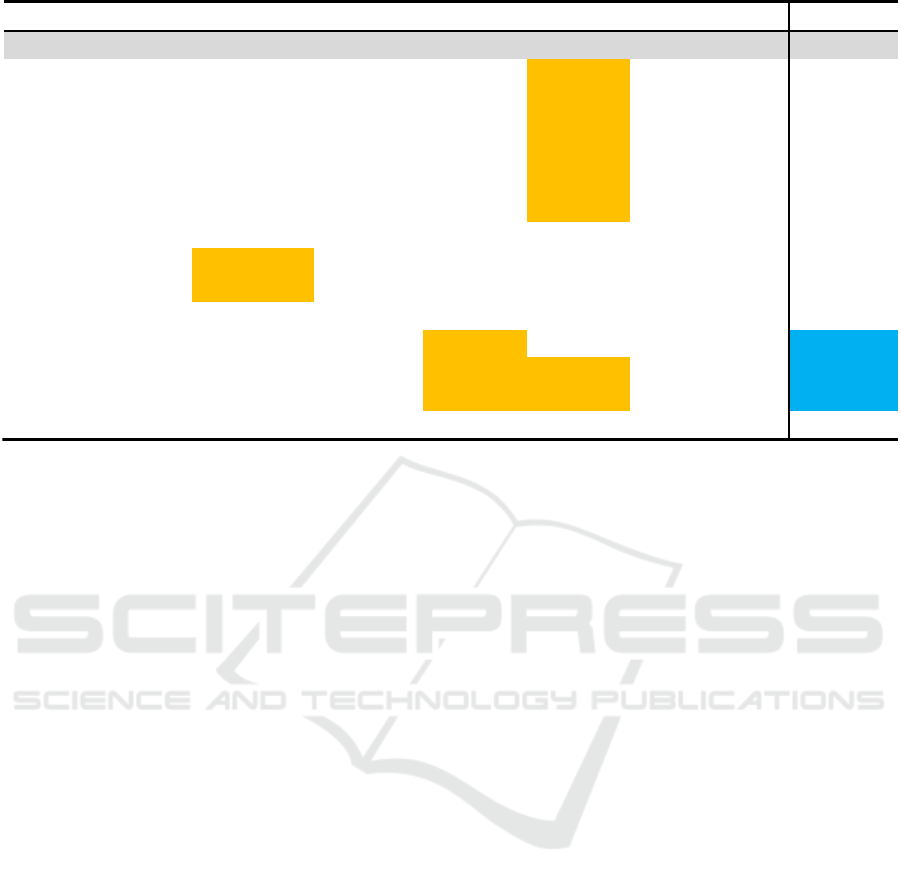
Figure 6 shows example perturbed cases for a

given test case. We perturbed the categorical features

marital and default with available values and used the

perturbation option from Figure 2 on the balance fea-

ture resulting in a total of 125 perturbed test cases, all

created by orange-level perturbation options. The ﬁrst

row in the table represents the original test case which

the model predicted with “no”, i.e., the customer will

probably not subscribe to a long-term deposit accord-

ing to the logistic regression model given the feature

values. 84 perturbed cases returned the same predic-

tion as the original case, 41 returned a changed pre-

diction and require further examination.

The ﬁrst six perturbed test cases shown in Figure

6 were generated by the perturbation option shown

in Figure 2. Adding and subtracting a small number

to the balance does not change the original predic-

tion and is, therefore, no problem for reliability. The

next two perturbed cases were generated by chang-

ing the marital feature with the other two available

values, “married” and “divorced”. This perturbation

does also not change the prediction and is, therefore,

no cause for concern regarding the reliability. The

next shown perturbed case changes the feature if a

customer has currently a credit in default, with the al-

lowed values “yes” and “no”. Applying this perturba-

tion option changes the original prediction from “no”,

the customer will not subscribe to a long-term deposit,

to “yes”, the customer will subscribe to a long-term

deposit. This means that if our potential new cus-

tomer had any credit in default, this would change the

prediction. This small change of input values, which

could be the actual case considering that the poten-

tial customer could have had a loan in default at an-

other bank without the organization knowing, means

that the analyst should probably not blindly trust the

prediction of the model. The analyst should consider

contacting the customer despite the model having re-

turned a “no” prediction. The perturbation mode fur-

ther calculates all combinations of perturbation op-

tions and receives predictions for all the thus created

perturbed test cases for further analysis.

The last two perturbed test cases in Figure 6 show

the beginning of the combination of the default fea-

ture perturbation option with the 10 percent pertur-

bation on the balance feature, which also leads to a

prediction change.

DATA 2021 - 10th International Conference on Data Science, Technology and Applications

132

age

job

marital

education

default

balance

housing

…

prediction

technician

single

secondary

2143.00

yes

…

technician

single

secondary

2164.43

yes

…

technician

single

secondary

2121.57

yes

…

technician

single

secondary

2185.86

yes

…

technician

single

secondary

2100.14

yes

…

technician

single

secondary

2207.29

yes

…

technician

single

secondary

2078.71

yes

…

technician

married

secondary

2143,00

yes

…

technician

divorced

secondary

2143,00

yes

…

technician

single

secondary

yes

2143,00

yes

…

yes

technician

single

secondary

yes

2164.43

yes

…

yes

technician

single

secondary

yes

2121.57

yes

…

yes

…

Figure 6: Perturbed test cases for the predictive model over the banking dataset.

The examples shown in Figure 6 were created by

orange-level perturbation options. These perturbation

options may change the prediction of a created per-

turbed test case due to reaching a label border in the

feature space. A red-level perturbation option should

not change the prediction in any case, since the real-

world value, perturbed with this option, is anywhere

within the perturbed range. An example is a value

measured by a sensor with a given interval for the sen-

sor accuracy; the real value lies within the margins of

the sensor accuracy. If a red-level perturbation option

changes a prediction, the prediction is not reliable.

The second approach, i.e., using local quality

measures, was also applied to the test case shown in

the example in Figure 6. We calculated the local accu-

racy for the test case in order to judge the prediction.

The overall accuracy of the model is about 78%. The

local accuracy is calculated based on the 1500 nearest

training set neighbors, as measured using Euclidean

distance, and has a value of 93%. That value means

that the subspace of the model that is considered has

a better performance than the overall performance of

the used classiﬁer. Since the overall performance of

the model is sufﬁcient for the analysis, there is lit-

tle doubt about reliability from the point of view of

this approach. Having local areas which have a bet-

ter accuracy than the global accuracy means, in turn,

that there are also areas and, consequently, test cases

where the local accuracy is worse, constituting a po-

tential problem for reliability.

7 SUMMARY AND FUTURE

WORK

In this paper, we introduced a reference process for

judging the reliability of classiﬁcation results over

structured data. We used the CRISP-DM and ex-

plained which tasks need to additionally be performed

in each of the six stages of CRISP-DM in order

to arrive at predictive analytics applications that al-

low for assessing the reliability of individual predic-

tions. Different data sources and their preparation

have different reliability-related information associ-

ated, which can be used in subsequent stages to con-

ﬁgure reliability-checking approaches. After the de-

ployment of the model, these approaches can be used

to judge the reliability of the predictions. The de-

scribed tasks in the data understanding, data prepa-

ration, and modeling stages must be performed once

for every use case. Gathered information and deﬁned

reliability-checking approaches are then examined if

they are appropriate to judge the reliability for the

use case during the evaluation phase. Once receiv-

ing predictions for new test cases, analysts can use

the previously speciﬁed approaches to judge the reli-

ability of individual predictions. The judgment is per-

formed for each individual case. Obtaining additional

information about the reliability of individual predic-

tions requires additional effort but improved reliabil-

ity will beneﬁt decision-makers in critical business

decisions. In this paper, we described the reference

process using a classiﬁcation example over structured

data, but we will investigate applications of the ref-

A Reference Process for Judging Reliability of Classiﬁcation Results in Predictive Analytics

133

erence process with other machine-learning methods,

e.g., regression or clustering, and different sorts of in-

put data, e.g., images, videos, and natural-language

text, in future work. A knowledge graph may serve

for the documentation of the knowledge regarding the

proper selection of the approach for reliability check-

ing.

REFERENCES

Barr, E. T., Harman, M., McMinn, P., Shahbaz, M., and

Yoo, S. (2015). The Oracle Problem in Software Test-

ing: A Survey. IEEE Trans. Software Eng., 41(5):507–

525.

Caetano, N., Cortez, P., and Laureano, R. M. S. (2014).

Using Data Mining for Prediction of Hospital Length

of Stay: An Application of the CRISP-DM Method-

ology. In Cordeiro, J., Hammoudi, S., Maciaszek,

L. A., Camp, O., and Filipe, J., editors, Enterprise

Information Systems - 16th International Conference,

ICEIS 2014, Lisbon, Portugal, April 27-30, 2014, Re-

vised Selected Papers, volume 227 of Lecture Notes

in Business Information Processing, pages 149–166.

Springer.

Capra, A., Castorina, A., Corchs, S., Gasparini, F., and

Schettini, R. (2006). Dynamic Range Optimization

by Local Contrast Correction and Histogram Image

Analysis. In 2006 Digest of Technical Papers Inter-

national Conference on Consumer Electronics, pages

309–310, Las Vegas, NV, USA. IEEE.

Chen, T. Y., Kuo, F.-C., Liu, H., Poon, P.-L., Towey, D.,

Tse, T. H., and Zhou, Z. Q. (2018). Metamorphic Test-

ing: A Review of Challenges and Opportunities. ACM

Comput. Surv., 51(1):4:1–4:27.

Cheney, E. W. and Kincaid, D. R. (2012). Numerical math-

ematics and computing. Cengage Learning.

Cruz, R. M. O., Sabourin, R., and Cavalcanti, G. D. C.

(2018). Dynamic classiﬁer selection: Recent advances

and perspectives. Inf. Fusion, 41:195–216.

da Rocha, B. C. and de Sousa Junior, R. T. (2010). Identify-

ing bank frauds using CRISP-DM and decision trees.

International Journal of Computer Science and Infor-

mation Technology, 2(5):162–169.

Didaci, L., Giacinto, G., Roli, F., and Marcialis, G. L.

(2005). A study on the performances of dynamic

classiﬁer selection based on local accuracy estimation.

Pattern Recognit., 38(11):2188–2191.

Guo, H., Shi, W., and Deng, Y. (2006). Evaluating sen-

sor reliability in classiﬁcation problems based on evi-

dence theory. IEEE Trans. Syst. Man Cybern. Part B,

36(5):970–981.

Hevner, A. R., March, S. T., Park, J., and Ram, S. (2004).

Design science in information systems research. MIS

quarterly, pages 75–105.

Moreira, D., Furtado, A. P., and Nogueira, S. C. (2020).

Testing acoustic scene classiﬁers using Metamorphic

Relations. In IEEE International Conference On Ar-

tiﬁcial Intelligence Testing, AITest 2020, Oxford, UK,

August 3-6, 2020, pages 47–54. IEEE.

Moro, S., Cortez, P., and Rita, P. (2014). A data-driven

approach to predict the success of bank telemarketing.

Decis. Support Syst., 62:22–31.

Moro, S., Laureano, R., and Cortez, P. (2011). Using data

mining for bank direct marketing: An application of

the crisp-dm methodology. Publisher: EUROSIS-ETI.

Moroney, N. (2000). Local Color Correction Using Non-

Linear Masking. In The Eighth Color Imaging Confer-

ence: Color Science and Engineering Systems, Tech-

nologies, Applications, CIC 2000, Scottsdale, Ari-

zona, USA, November 7-10, 2000, pages 108–111.

IS&T - The Society for Imaging Science and Tech-

nology.

Reimer, U., T

odtli, B., and Maier, E. (2020). How to Induce

Trust in Medical AI Systems. In Grossmann, G. and

Ram, S., editors, Advances in Conceptual Modeling -

ER 2020 Workshops CMAI, CMLS, CMOMM4FAIR,

CoMoNoS, EmpER, Vienna, Austria, November 3-6,

2020, Proceedings, volume 12584 of Lecture Notes in

Computer Science, pages 5–14. Springer.

Saha, P. and Kanewala, U. (2019). Fault Detection Ef-

fectiveness of Metamorphic Relations Developed for

Testing Supervised Classiﬁers. In IEEE International

Conference On Artiﬁcial Intelligence Testing, AITest

2019, Newark, CA, USA, April 4-9, 2019, pages 157–

164. IEEE.

Segura, S., Fraser, G., S

anchez, A. B., and Cort

es, A. R.

(2016). A Survey on Metamorphic Testing. IEEE

Trans. Software Eng., 42(9):805–824.

Vriesmann, L. M., Jr, A. S. B., Oliveira, L. S., Koerich,

A. L., and Sabourin, R. (2015). Combining overall

and local class accuracies in an oracle-based method

for dynamic ensemble selection. In 2015 International

Joint Conference on Neural Networks, IJCNN 2015,

Killarney, Ireland, July 12-17, 2015, pages 1–7. IEEE.

Wirth, R. and Hipp, J. (2000). CRISP-DM: Towards a Stan-

dard Process Model for Data Mining. page 11.

Woods, K. S., Kegelmeyer, W. P., and Bowyer, K. W.

(1997). Combination of Multiple Classiﬁers Using

Local Accuracy Estimates. IEEE Trans. Pattern Anal.

Mach. Intell., 19(4):405–410.

Xie, X., Ho, J. W. K., Murphy, C., Kaiser, G. E., Xu, B., and

Chen, T. Y. (2011). Testing and validating machine

learning classiﬁers by metamorphic testing. J. Syst.

Softw., 84(4):544–558.

DATA 2021 - 10th International Conference on Data Science, Technology and Applications

134