Profit Maximized Network Optimization at SAP System:

A Real-life Implementation in Cement Industry

Eren Esgin

1,2 a

, Volkan Ozay

and Gorkem Ozkan

AI Research, MBIS R&D Center, Istanbul, Turkey

Informatics Institute, Middle East Technical University, Ankara, Turkey

Keywords: Business Planning, Integer Programming, Network Optimization, Profit Maximization, SAP, Variance

Analysis, What-if Scenario Evaluation.

Abstract: What if we told you that “you already have 27% of net profit trapped in your misleading business”? As

common de facto state in production planning, subjective human judgments play a significant role on demand

point:plant assignments at product replenishment and this is mostly driven by myopic transportation

minimization paradigm, disregarding production and profitability determinants. In this paper, we propose an

integer programming characterized Network Optimization solution to find global optimal assignments that

maximize the profitability in terms of contribution margin or net profit by taking sales, transportation and

production planning perspectives into account and concerning potential capacity constraints. According to the

experimental results obtained at a real-life implementation in cement industry, Network Optimization solution

increases contribution margin by an average value of 6.33% and net profit by 26.3%. Moreover, proposed

solution architecture promises a seamless network optimization experience over a large canvas that

wholistically integrates SAP system, optimization logic and Microsoft Power BI tiers. As a result, our clients

can concentrate on more value adding operations such as variance analysis and what-if scenario evaluation

rather than manual, time consuming and error-prone data preparation.

1 INTRODUCTION

In the last year,

COVID19

imposed Schumpeter's gale

“creative destruction” like business transformation to

the organizations all around the world to adapt to the

concept drifts and uncertainties emerged at the

business environment. In this context, business

planning solutions are crucial actors at this era such

that, these products provide the capabilities to

simulate various what-if scenarios to monitor

potential bottlenecks emerged at organizational

scarce sources, e.g. liquid capital, workforce and

installed capacity, and to proactively response to

customer demand fluctuations by unmanned

sustainable business models.

Seemingly, one of the major issues at business

planning solutions is the satisfaction of customer

demand by the most appropriate production facility.

As the state-of-art, subjective human judgments on

demand point:plant assignments at product

replenishment play a vital role and this assignment is

https://orcid.org/0000-0002-5454-4244

driven by biased aspect solely based on transportation

minimization. Additionally, hand simulation

performed by process owners requires more effort on

data preparation. Hence less variance analysis and

what-if scenario evaluation are performed.

Network Optimization solution aims to find

global optimal demand point:plant assignments that

maximize total net profit or contribution margin

objective value according to planned sales volume,

unit sales price, unit transportation cost, unit variable

and fixed production cost. Additionally, capacity

constraints planned at plant or plant-product detail

levels and demand satisfaction constraints are other

determinants of the proposed approach.

Respectively, Network Optimization solution

promises the harmonization of mathematical

modelling with human insights. Hence, the myopic

aspect over transportation minimization is extended

towards profitability maximization and production

capacity. As a result, process owners dedicate more

effort on variance analysis and different what-if

752

Esgin, E., Ozay, V. and Ozkan, G.

Proﬁt Maximized Network Optimization at SAP System: A Real-life Implementation in Cement Industry.

DOI: 10.5220/0010618507520760

In Proceedings of the 18th International Conference on Informatics in Control, Automation and Robotics (ICINCO 2021), pages 752-760

ISBN: 978-989-758-522-7

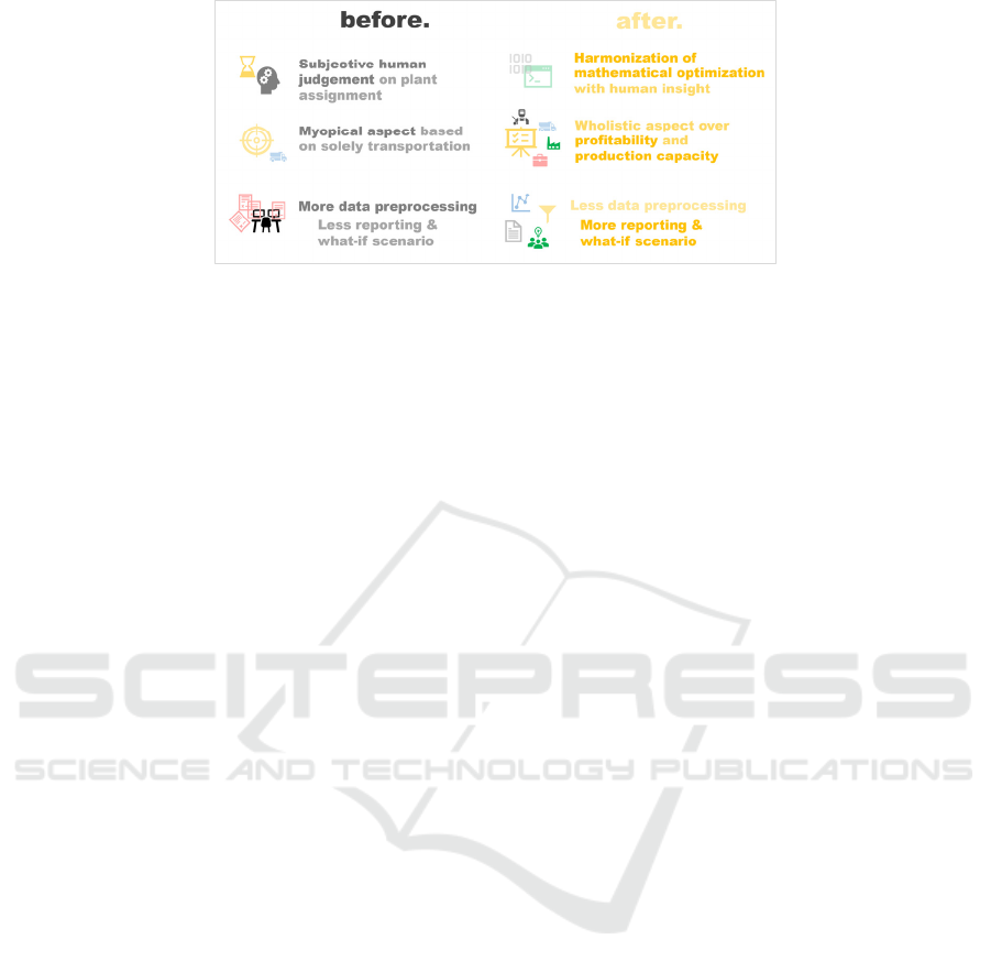
Figure 1: Fit Gap Analysis for Network Optimization Solution.

scenarios evaluation. According to business

requirement analysis and the leverage effect promised

by Network Optimization solution, fit gap analysis is

performed as given in Figure 1.

The paper is organized as follows. Section 2

reviews the related work about network optimization

and transportation minimization applications. Section

3 explains Network Optimization solution within the

context of solution architecture and major phases of

the proposed approach. Section 4 discusses the

experimental results obtained at a real-life

implementation in cement industry. The conclusion

and future work are summarized in Section 5.

2 LITERATURE REVIEW

Literature review section fundamentally concentrates

on the applications of maximizing profits, network

optimization and minimizing transportation costs in

various manufacturing industries.

Billal, Islam, Alam and Hossain (2015) considers

the time value of money, cost variance due to the

transportation mode and responsive supply chain in a

single model. The multi-stage supply chain network

design (SCND) model is designed for the

organization that operates in cement industry and

meets the customer demand at the divisional markets

in Bangladesh. The Mixed Integer Linear

Programming (MILP) is used in the SCND model.

Sulistyo, Herryandie and Jonrinaldi (2019) explains

system modelling and the required parameters to

compile the mathematical model which is applied to

computer simulation used by the logistics manager to

make operational decisions. Dikos and Spyropoulou

(2013) proposes a platform for optimization supply

chains and planning that uses mathematical

programming. The underlying platform uses a series

of nested mathematical programs to model the supply

chain operations. This platform determines optimal

operational response to fluctuations in both demand

and production, and then performs mid and long-term

planning in the context of what-if scenario evaluation.

Das, Adnan, Hassan and Rahman (2017) aims to

understand the terms of logistics cost and

optimization techniques by a cost-optimizing solver

developed in Microsoft Excel. As a result of using

optimization tools and techniques, it is shown in a

comparative way that an organization can reduce

overall logistics costs by identifying cost factors and

using them correctly. Chukwuma and Chukwuma

(2015) designs a model for capacity planning and

scheduling using Linear Programming. The

underlying model suggests the most efficient route

that minimizes transportation costs for the cement

producers.

The operations management technique of linear

programming (LP) is integrated into a cost accounting

information system in Excel as an add-in to maximize

profit and minimize cost in (Togo, 2005). Similarly,

a global supply chain optimization model that

maximizes the after-tax profits of a multinational

corporation is introduced in (Vidal & Goetschalckx,

2001). This research helps on simultaneous

consideration of transferring prices, transportation

cost allocation, inventory costs and their impact on

the selection of international transportation modes.

Oladejo, Abolarinwa, Salawu and Lukman (2019)

examines to maximize the profit and reduce the costs

using linear programming. As a result of this study,

the underlying mathematical model determines which

products should be produced and sold to maximize

profit.

Vimal, Rajak and Kandasamy (2019) aims to

maximize the total monetary gain and minimizing

pollution such that, the profits generated by the sale

of both reused and manufactured products, profits

gained from recycling units, cost of processing, setup,

and repair at the intake nodes, and transportation costs

are totally considered during the linear programming

model design. In (Samani & Mottaghi, 2006), the

optimum design of municipal water distribution

Proﬁt Maximized Network Optimization at SAP System: A Real-life Implementation in Cement Industry

753

networks for a single loading condition is determined

by the integer linear programming technique to

design a water distribution system that satisfies all

required constraints with a minimum total cost.

Kostin et al. (2018) presents a mathematical approach

with MILP formulation for optimizing and planning

Brazilian bioethanol supply chains. This approach

aims to maximize the net present value of the entire

supply chain of the sugar and bioethanol industry in

Brazil, and proposes the technology chosen for the

optimal configuration of a bioethanol network and the

flows of all raw materials and final products involved.

3 PROPOSED APPROACH

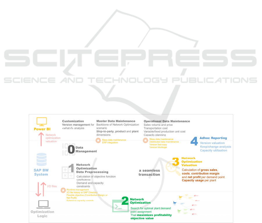
3.1 Solution Architecture

Solution architecture of Network Optimization

solution consists of three layers: SAP BW system,

optimization logic and Microsoft Power BI.

SAP BW system is the core component of

Network Optimization solution. Major use cases such

as data management, network optimization data pre-

processing, optimization valuation and adhoc

reporting are executed at this layer. The

corresponding components and transactions are

developed in ABAP programming language.

Optimization logic layer holds the network

optimization mathematical modelling. This model

searches for global optimal demand point:plant

assignments that maximize the objective function, i.e.

contribution margin or net profit. The corresponding

integer programming (IP) based mathematical model

is developed in R programming language. Majorly,

lpSolve and dplyr packages are implemented.

Lastly, Power BI is the presentation layer that

demonstrates various dashboards such as income

statement and product or customer-based profitability

analysis reports with zoom-in/out functionalities.

These dashboards are based on the network

optimization valuation view held at SAP BW system.

Proposed solution architecture is given in Figure 2.

3.2 Phases

Network Optimization solution is composed of three

major phases: data management, optimization and

adhoc reporting. These phases are explained in

detailed at the following sections.

3.2.1 Data Management

In data management phase, required input data for

optimization is maintained in three ways such as

customization, master and planning data.

Network Optimization solution is based upon a

what-if paradigm which manages different potential

circumstances (or variants) at planning data, e.g. sales

volume, sales price, transportation cost and

feasibility, production cost and feasibility, and lastly

capacity constraints. Hence customization data is

used for an active version management. In the context

of version management, it is possible to make before

versus after simulation variance analysis such that,

while before simulation typed versions hold the

process owner’s direct insights about demand

point:plant assignments as the ground truth, after

Figure 2: Proposed Solution Architecture. Process enhancements at the corresponding planning phases are denoted by yellow

stars.

ICINCO 2021 - 18th International Conference on Informatics in Control, Automation and Robotics

754

simulation typed versions purely reflect the global

optimal assignments obtained by the underlying

network optimization runs. As the relation between

these two version types, demand point:plant

assignments proposed at before simulation version is

used as the baseline for unit transportation cost

determination at delivered sales price conversion.

As the enhancement of Network Optimization

solution, there is an objective function type feature at

version customization step. This feature is used for

designating objective function applied at network

optimization such as contribution margin or net profit

maximization. Distinctions and relations between

before and after simulation type versions are given in

Figure 3.

Master data constitutes the backbone of the proposed

approach such that, it contains major planning

dimensions, i.e. ship-to-party, product and plant.

While these dimensions can be maintained

individually via the corresponding data management

user interfaces (UIs), it is also possible to export mass

master data and import actual dimension members

from SAP ERP system. Respectively, ship-to-party is

a kind of dynamic dimension. Therefore, these

alternative mass data maintenance interfaces and

transactions are more effective for keeping ship-to-

party dimension up-to-date. Details about planning

dimensions are given as below:

 Ship-to-party dimension holds the major features

of valid customers such as name, region, city, city

district and micro-market.

 Product dimension contains the name, product

type (bag or bulk cement) and segment (e.g.

strength level bag cement,

C2 strength level bulk

cement etc.) features.

 Plant dimension contains the name and active

plant indicator features.

Planning data relatively reflects the what-if

circumstances for the corresponding version. These

circumstances can be designated by sales (e.g. sales

volume and price), transportation (e.g. transportation

cost) and production (e.g. variable or fixed production

costs, capacity constraints at plant or plant-product

detail levels) functional areas. Details about planning

data management are given below:

 Sales volume (vol) and price (prc) planning step

instantiates potential demand points (dp) which

imply valid combinations of ship-to-party (STP

set) and product (PRD set) dimensions as given in

Equations 1 and 2.

According to simulated/preset indicator at sales

planning step, it is possible to determine whether

the underlying demand point will be covered by

network optimization or assigned to an apriori

plant predefined at before simulation typed

version. Additionally, sales process owner plans

the exwork prices according to the unit

transportation cost retrieved from before

simulation typed version of the corresponding

period and the delivered sales price determined at

sales contract document.

 At transportation cost (trs) planning step,

estimated unit transportation cost is planned on

ship-to-party (dp

.stp), product type (dp

.prd_typ)

and plant basis (plt) as given in Equation 3. In the

case of infeasible combinations that exceed the

maximum distance threshold (approximately 400

kilometers), unit transportation cost is manually

set as a big M value, e.g. one million ₺ per ton.

 Variable production cost (vpc) planning step

holds the estimated variable production cost on

product (dp

.prd) and plant (plt) basis as given in

Equation 4. This variable cost component reflects

the production cost drivers that are directly

correlated with the production volume such as

direct material cost calculated according to the bill

of material (BOM). In the case of infeasible

production capability, unit variable production

cost is manually set as a big M value, e.g. one

million ₺ per ton.

Figure 3: Distinctions and Relations between Before and After-simulation Typed Versions.

Proﬁt Maximized Network Optimization at SAP System: A Real-life Implementation in Cement Industry

755

 Fixed production cost (fpc) planning step holds

the estimated fixed production cost on plant (plt)

basis as given in Equation 5. This fixed cost

component reflects the production cost drivers

that are not affected by the production volume but

correlated with installed capacity such as

amortization and direct labor cost calculated

according to the production routing.

Sample planning user interfaces for sales,

transportation and production planning steps are

given in Appendix. Additionally, capacity constraints

are other determinants handled at data management

phase:

 Plant-based capacity planning step includes plant

utilization rate, total capacity, and product type

(bag or bulk) capacity figures on plant (plt) basis.

These capacity figures per plant are revaluated on-

the-fly by the utilization rate input.

 At product-based capacity planning step, capacity

figures are specifically planned at product

(dp

.prd) and plant (plt) details. These product

relevant capacity figures per plant are calculated

on-the-fly by the utilization rate planned at

previous plant-based capacity planning step.

3.2.2 Optimization

Optimization phase consists of three steps namely

network optimization data pre-processing,

optimization and valuation as shown in Figure 2.

In network optimization data pre-processing,

three different input data, which are objective

function coefficients (coef

dpi,pltj

) for all demand

point:plant combinations, demand satisfaction and

capacity constraints, are all generated by using

customization, master and planning data for the

underlying version.

In the case of contribution margin maximization

objective function preference for the underlying

version, objective function coefficient (coef

dpi,pltj

Equations 3-4) implies the sum of gross sales

(Equation 2), transportation cost (Equation 3) and

variable production cost (Equation 4) for each

demand point(dp):plant(plt) combination. In the case

of net profit maximization objective function

preference, fixed production cost is also considered at

objective function calculation as given in Equation 5.

Underlying objective function coefficient calculation

steps are given at Equations 2-5:

DP = STP × PRD

(1)

gr_sl

dpi

= vol

dpi

× prc

dpi

(2)

coef

dpi,pltj

= gr_sl

dpi

−

vol

dpi

× trs

dpi.stp,dpi.prd_typ,pltj

(3)

coef

dpi,pltj

= coef

dpi,pltj

−

vol

dpi

× vpc

dpi.prd,pltj

(4)

coef

dpi,pltj

= coef

dpi,pltj

−

vol

dpi

× fpc

pltj

(5)

Demand satisfaction constraint holds the planned

sales volumes of the demand points that are set as

simulated at simulated/preset indicator. In other

words, preset demand points are omitted at demand

satisfaction constraint. This constraint line item also

holds additional information such as ship-to-party,

product and product type features of the underlying

demand point. As a restriction, total volume of

demand point must be replenished by a single plant.

Since underlying sales volume cannot be distributed

over multiple plants, Network Optimization solutions

evolves towards an integer programming (IP)

characterized mathematical model.

Capacity constraints reflect the rationale of scarce

production source of production facilities. These

constraints can be designated at four distinct detail

levels: plant, product type (bag/bulk) and plant,

product segment and plant, and lastly product and

plant via the capacity planning steps introduced in

Section 3.2.1. Additionally, sales volumes of preset

typed demand points are subtracted from the

corresponding capacity figures before network

optimization run.

At optimization step, linear programming

algorithm is applied to achieve profit maximization

and solve the underlying assignment problem. This

algorithm retrieves all simulated type demand

point:plant combinations as candidate solutions and

takes production capacity and demand satisfaction

constraints into account. After data pre-processing

step, the input data calculated at SAP BW system

layer for the underlying version is transferred to

optimization logic layer as shown in Figure 2.

Respectively, optimization step aims to maximize

total objective function value, i.e. contribution margin

or net profit. In this aspect, assignment of a demand

point dp

to a plant plt

implies the demand

satisfaction for dp

and a local increase at objective

function value worth of the unit margin value realized

by dp

:plt

assignment calculated at Network

Optimization data pre-processing step. On the

contrary, a portion of capacity figures related to

demand point dp

and plant plt

is diminished due to

this demand satisfaction.

Technically, we positioned an integer

programming characterized mathematical model to

satisfy each demand point with exactly one plant in

an optimality fashion such that, it maximizes total

contribution margin or net profit with respect to any

given number of plants and demand points.

ICINCO 2021 - 18th International Conference on Informatics in Control, Automation and Robotics

756

Accordingly, lpSolve package has several input

arguments to work appropriately such as objective

function vector that is essentially the target for our

problem required to be expressed in a mathematical

way, and a constraint matrix to consider the

constraints given above and totally satisfy them

correctly. The constraint matrix is composed of two

partitions: the demand constraint determined for each

simulated typed demand point and capacity

constraints planned at any detail levels. Finally, for

every constraint we shall have an operand vector to

express the limits in a mathematical manner, e.g., =

or ≤ etc., and the constraint figures that can be

considered as right-hand side (RHS) vector that holds

the threshold values about the underlying constraints.

After the completion of every aspect of the constraint

side, optimization step is ready to use

lpSolve

functions, e.g.

LP, to obtain the optimal results

according to the input objective function coefficients

and constraints.

Once mathematical model returns the global

optimal solution vector, we convert the demand

point:plant optimal assignments to a 2D matrix and

traverse at this matrix to obtain 1-valued assignments

with disregarding 0-valued elements. Finally, these

assignments are transferred to SAP BW system layer

for network optimization valuation step as shown in

Figure 2. Additionally, underlying input data, i.e.

objective function coefficients, demand satisfaction

and capacity constraints, and optimal solution are also

saved as local files at SAP file directory, aka

AL11

transaction.

The underlying mathematical model is given

below as Algorithm 1.

Algorithm 1: Integer Programming (IP) Characterized

Network Optimization Mathematical Model.

𝑀𝐴𝑋



𝑐𝑜𝑒𝑓

,

×𝑖

,



s.t:



𝑣𝑜𝑙



𝑖

,

≤ 𝑐𝑝𝑐𝑡𝑦



𝑓𝑜𝑟 ∀𝑝𝑙𝑡𝑗 ∈ 𝑃𝐿𝑇



𝑣𝑜𝑙



𝑖

,

≤𝑐𝑝𝑐𝑡𝑦

,_

𝑖𝑓 𝑑𝑝𝑖.𝑝𝑟𝑑_𝑡𝑦𝑝 = 𝑝𝑟𝑑_𝑡𝑦𝑝𝑘



𝑣𝑜𝑙



𝑖

,

≤𝑐𝑝𝑐𝑡𝑦

,_

𝑖𝑓 𝑑𝑝𝑖.𝑝𝑟𝑑_𝑠𝑒𝑔 = 𝑝𝑟𝑑_𝑠𝑒𝑔𝑘



𝑣𝑜𝑙



𝑖

,

≤𝑐𝑝𝑐𝑡𝑦

,

𝑖𝑓 𝑑𝑝𝑖. 𝑝𝑟𝑑 = 𝑝𝑟𝑑𝑘



𝑖

,



𝑓𝑜𝑟 ∀𝑑𝑝𝑖 ∈ 𝐷𝑃

𝑖

,

∈ {0, 1}

Line 1 represents objective function such that,

binary variable i

dpi,pltj

holds the underlying atomic

:plt

assignment decision and variable coef

dpi,pltj

unit contribution margin or net profit coefficient

calculated at network optimization pre-processing

step. Value of these coefficients are determined

according to the objective function type preference of

the underlying version. Lines 2-5 represent capacity

constraints determined at different plant and product

detail levels, i.e. plant, demand point product type

(dp

.prd_typ), product segment (dp

.prd_seg) or

product (dp

.prd). Respectively, Line 6 holds the

customer satisfaction determined for each simulated

typed demand point. The last line enhances integer

programming (IP) characteristic to the underlying

mathematical model.

After obtaining the optimal demand point:plant

assignment solution, valuation step calculates exact

gross sales, transportation cost, fixed and variable

production cost, contribution margin and net profit

values for each demand point via Equations 2-5.

According to the planning dimensions, e.g. ship-to-

party, plant and product, and the features of these

planning dimensions, e.g. city, city district, product

group, it is possible to analyse the network

optimization valuation by zoom-in/out functionality.

These figures are managed by version and

GUID (i.e.

a unique runtime identifier as shown in Figure 3) at

Network Optimization solution. Process owner can

compare different versions and network optimization

runs for the corresponding period by keep/change

variance analysis report. Finally, valuation figures of

the optimal network optimization run are transferred

to the adhoc reporting phase or Microsoft Power BI

layer as shown in Figure 2.

3.2.3 Adhoc Reporting

Adhoc reporting phase provides various reporting

functionalities to analyse the valuation figures for

each valid before or after simulation typed versions,

perform keep/change variance analysis among the

corresponding what-if scenarios and monitor capacity

consumptions at different plant and product detail

levels.

4 EXPERIMENTAL RESULTS

In the scope of pilot runs, Network Optimization

solution is implemented at one of our instalment-

based SAP clients operating in cement industry. This

leading organization has 6 plant facilities located in

Central Anatolia region in Turkey and replenishes

bag or bulk typed cement products to approximately

500 potential or actual ship-to-parties spread over

Ankara, Black Sea, Central and Eastern Anatolia

Proﬁt Maximized Network Optimization at SAP System: A Real-life Implementation in Cement Industry

757

regions. Current product portfolio consists of 11

product groups.

As the experimental analysis, we focus on two

months that are relatively sales intensive and

bottleneck periods, i.e. August 2020 and September

2020, respectively. These periods constitute of

approximately 350 demand points and 5 active

capacity constraints designated at different plant and

product detail levels as stated in Section 3.2.2. Due to

what-if scenario evaluation, we created 6 distinct

planning versions such that, two before simulation

typed versions with

yyyy_mm_B0 notation, two after

simulation typed versions with yyyy_mm_A1 notation

that maximize contribution margin and two after

simulation typed versions with

yyyy_mm_A2 notation

that maximize net profit. Experimental results can be

evaluated within two variance analysis: before versus

after and after versus after variance analysis.

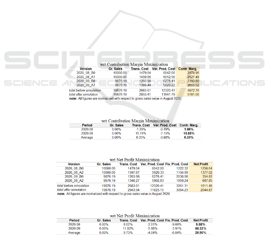
4.1 Before vs. After Variance Analysis

According to contribution margin maximization

objective preference, Network Optimization solution

promises adequate increase at the objective value by

an average value of 6.33% as shown in Table 1.

Although this improvement is degraded by the

indispensable increase at transportation cost

(approximately 6.35%), minimization of variable

product cost by an average value of 3.88%, which

constitutes the major portion of cost accrual, result in

improvement at total contribution margin (from

4872.8K ₺ to 5181K ₺).

Similarly, net profit maximized network

optimization increases the objective value by an

average value of 26.9% as shown in Table 2.

Although there happens a 9.73% increase at

transportation cost, this tendency is damped by

significant shrinkage at fixed and variable production

costs, i.e. 4.04% and 6.04% reductions respectively.

The mechanism emphasized at both what-if

scenarios is due to the fact that, while human insights

at before simulation typed version is myopically

based on transportation minimization, Network

Optimization solution provides a wholistic

perspective that considers both transportation and

production cost drivers at profitability. Respectively,

total (fixed and variable) production costs are

approximately 4.9 times higher than total

transportation costs. Hence, network optimization

tends to assign demand points to geographically far

Table 1a: Before vs. After Variance Analysis.

Table 1b: Nominal Variance per Period.

Table 2a: Before vs. After Variance Analysis.

Table 2b: Nominal Variance per Period.

ICINCO 2021 - 18th International Conference on Informatics in Control, Automation and Robotics

758

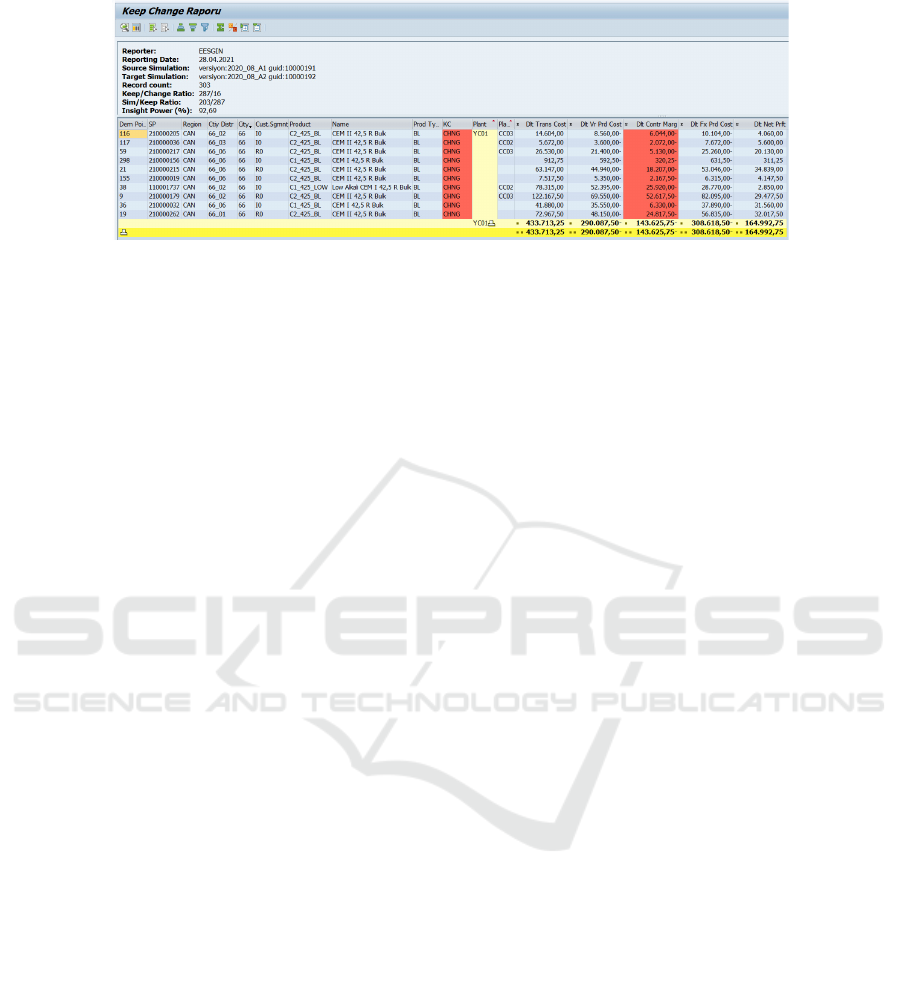
Figure 4: Keep Change Report for August 2020 period (variance analysis between 2020_08_A1 and 2020_08_A2).

and still feasible plants with high-tech production

lines. This high-tech notion implies lower

amortization costs, shorter standard production cycle

times and higher capacity utilizations.

4.2 After vs. After Variance Analysis

As stated in Section 3.2.2, Network Optimization

solution has a configurable objective function feature.

Hence, it is possible to perform keep change variance

analysis that emphasizes changing demand

point:plant assignments due to the effect of

contribution margin or net profit objective function

preference.

In this aspect, there happens interesting demand

point:plant assignment changes in August 2020

period as shown in Figure 4. 11 demand points in city

66 are priorly assigned to plant

YC01, which is also

located in city 66, at version

2020_08_A1. These

demand points are then assigned to geographically far

plants (e.g.

CC02 and CC03) at version 2020_08_A2.

According to these changing points, there raises an

opportunity cost of 433.7K ₺ in transportation cost

and 143.6K ₺ loss in contribution margin.

On the contrary, because of net profit maximizing

objective function preference at version

2020_08_A2,

it can evaluate further trade-offs potentially emerged

between transportation cost and fixed production cost

drivers such that, 143.6K ₺ loss at contribution

margin is amended by 308.6K ₺ gain at fixed

production cost. Due to the rationale of sunk costs

realized by production idle capacity in plant

YC01, i.e.

higher amortization cost, longer standard production

cycle times and lower capacity utilization,

replenishment of cement to the underlying 11 demand

points from geographically nearest plant turns into an

unprofitable status.

As the non-functional business requirement,

Network Optimization solution eliminates time-

consuming and erroneous hand simulation performed

by process owners at Microsoft Excel solver.

Accordingly, current total processing time is

dramatically lessened from 2 hours to 30 seconds at

the pilot runs.

5 CONCLUSIONS

This paper demonstrates Network Optimization

solution deployed at SAP system and proposed

solution architecture provides a seamless network

optimization experience over a large environment

orchestrating SAP system, optimization logic and

Microsoft Power BI layers. Correspondingly, the

underlying solution paradigm aims to find global

optimum demand point:plant assignments at product

replenishment that maximize total profitability in

terms of contribution margin or net profit with respect

to sales, transportation and production planning data

and concerning capacity and customer satisfaction

constraints.

As the current (as-is) situation, human judgments

is the major determinant in demand point:plant

assignments within a myopic aspect solely focusing

on transportation minimization. Additionally, hand

simulation executed at Microsoft Excel solver is a

time consuming and error-prone procedure such that,

less effort is dedicated to more value adding

operations. On the contrary, Network Optimization

solution provides a wholistic aspect towards profit

maximization by the leverage effect of mathematical

modelling. Hence, process can focus on variance

analysis and different what-if scenarios evaluation.

According to experimental results, Network

Optimization solution increases the contribution

margin by an average value of 6.33% and net profit

by 26.9%. Additionally, configurable objective

function feature at version management provides an

effective after versus after variance analysis that

compares different what-if scenarios highlighting

potential trade-offs between transportation and

production cost drivers. As the future work, we plan

Proﬁt Maximized Network Optimization at SAP System: A Real-life Implementation in Cement Industry

759

to spread proposed solution towards different

industries confronting similar network optimization

bottlenecks.

REFERENCES

Billal, M., Islam, M., Alam, S. & Hossain M. (2015).

Optimal Supply Chain Network Opportunities: The

Case of Bangladesh. World Journal of Social

Sciences 5.3

Chukwuma, N. K., & Chukwuma E. (2015). Optimizing

Cement Distribution in the Nigerian Cement

Manufacturing Industry: The Case of Cement

Distribution from Selected Firms to Markets in Ebonyi

State. International Journal of Research in Business

Management 3.2:35-64.

Das, A., Adnan, T. M., Hassan, S. & Rahman K. M. (2017).

Analysing Logistics Cost Factors and Developing Cost

Optimization Tools and Techniques for a Cement

Industry (Case Study: Lafarge Surma Cement Ltd).

International Research Journal of Engineering and

Technology (IRJET) 4.04:1504.

Dikos, G., & Spyropoulou, S. (2013). Supply Chain

Optimization and Planning in Heracles General

Cement Company. Interfaces 43.4:297-312.

Kostin, A., Macowski D. H., Pietrobelli, J. M. T. A.,

Guillen-Gonsalbez, G., Jimenez, L., & Ravagnani, M.

A. S. S. (2018). Optimization-Based Approach for

Maximizing Profitability of Bioethanol Supply Chain in

Brazil. Computers & Chemical Engineering 115:121-

132.

Oladejo, N. K., Abolarinwa, A., Salawu, S.O. & Lukman,

A. F. (2019). Optimization Principle and Its’ Applica-

tion in Optimizing Landmark University Bakery

Production Using Linear Programming. International

Journal of Civil Engineering and Technology (IJCIET)

10.2:183-190.

Samani, H. M. V., & Mottaghi, A. (2006). Optimization of

Water Distribution Networks Using Integer Linear

Programming. Journal of Hydraulic Engineering

132.5:501-509.

Sulistyo, D. E., Herryandie, A. & Jonrinaldi (2019).

Inventory and Transportation Model for Decision

Making in Cement Industry (Case study at PT Semen

Padang). IOP Conference Series: Materials Science

and Engineering. 505:1.

Togo, D. F. (2005). Integrating Operations Management

into Cost Systems: An Accounting Approach to Linear

Programming. Journal of Business Case Studies

(JBCS) 1.4:27-32.

Vidal, C. J., & Goetschalckx, M. (2001). A Global Supply

Chain Model with Transfer Pricing and Transportation

Cost Allocation. European Journal of Operational

Research 129.1:134-158.

Vimal, K. E. K., Rajak, S. & Kandasamy, J. (2019).

Analysis of Network Design for a Circular Production

System Using Multi-Objective Mixed Integer Linear

Programming Model. Journal of Manufacturing

Technology Management, 30.3:628-646.

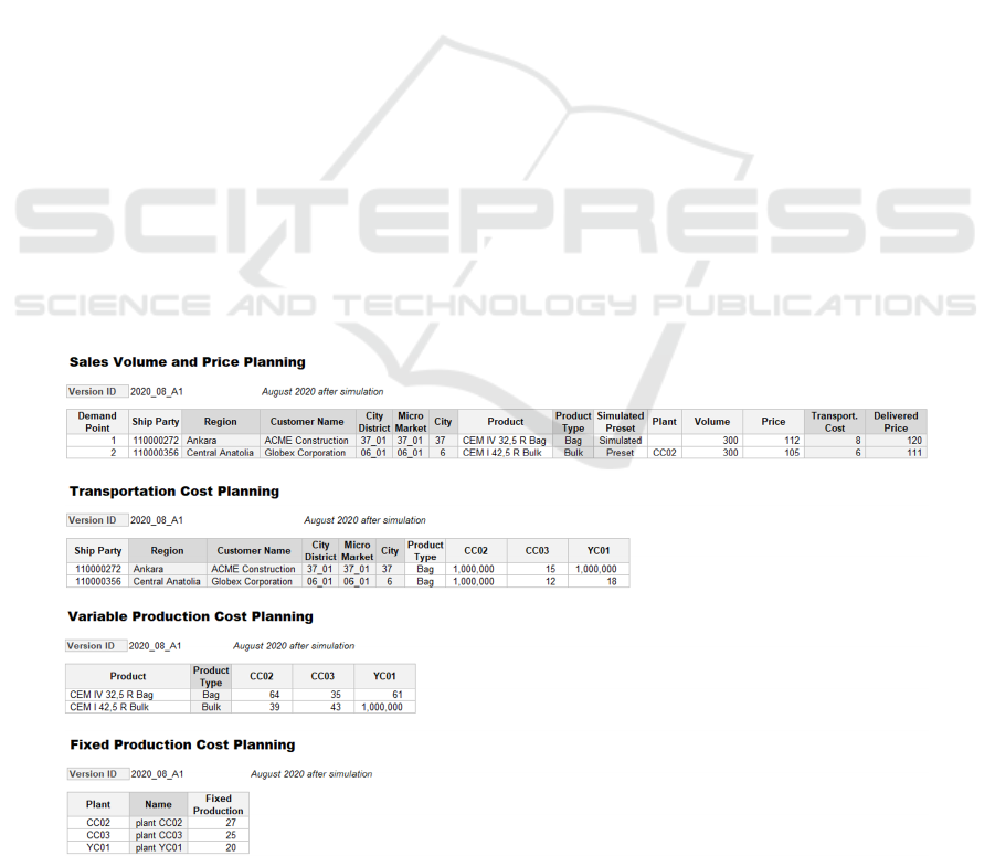
APPENDIX

Sample planning user interfaces, e.g. sales volume

and price, transportation cost, variable and fixed

product cost planning, are given in Figure 5.

Figure 5: Sample Planning User Interfaces maintained via a version ID parameter. While editable fields are shown in light

grey shade, the fields automatically extracted from planning dimensions’ master data are given in dark gray color.

ICINCO 2021 - 18th International Conference on Informatics in Control, Automation and Robotics

760