
Deep Reinforcement Learning for Dynamic Power Allocation in Cell-free
mmWave Massive MIMO
Yu Zhao
a
, Ignas Niemegeers
b
and Sonia Heemstra de Groot
c
Department of Electrical Engineering, Eindhoven University of Technology, Eindhoven, The Netherlands
Keywords:
Cell-free Massive MIMO, Deep Reinforcement Learning, Deep Q-Network, Power Allocation.
Abstract:
Numerical optimization has been investigated for decades to solve complex problems in wireless communi-
cation systems. This has resulted in many effective methods, e.g., the weighted minimum mean square error
(WMMSE) algorithm. However, these methods often incur a high computational cost, making their applica-
tion to time-constrained problems difficult. Recently data-driven methods have attracted a lot of attention due
to their near-optimal performance with affordable computational cost. Deep reinforcement learning (DRL) is
one of the most promising optimization methods for future wireless communication systems. In this paper,
we investigate the DRL method, using a deep Q-network (DQN), to allocate the downlink transmission power
in cell-free (CF) mmWave massive multiple-input multiple-output (MIMO) systems. We consider the sum
spectral efficiency (SE) optimization for systems with mobile user equipment (UEs). The DQN is trained
by the rewards of trial-and-error interactions with the environment over time. It takes as input the long-term
fading information and it outputs the downlink transmission power values. The numerical results, obtained for
a particular 3GPP scenario, show that DQN outperforms WMMSE in terms of sum-SE and has a much lower
computational complexity.
1 INTRODUCTION
Massive multiple-input multiple-output (MIMO)
(Larsson and Edfors, 2014) and the use of mmWave
spectrum, have been widely recognized as key to in-
creasing the system capacity by an order of magnitude
compared to present sub-6 GHz networks (Busari and
Huq, 2018). This is because of the larger band-
width available in the mmWave spectrum and the
significantly higher spectral efficiency (SE) that can
be achieved with massive MIMO (Andrews and G.,
2014).
In massive-MIMO, a base station (BS), equipped
with a very large antenna array, serves simultaneously
multiple user-equipments (UEs), using the same time-
frequency resource. The number of antennas should
significantly exceed the number of UEs. Further gains
can be obtained by spreading the antennas over multi-
ple geographically distributed access points (APs), in-
stead of concentrating them in a single BS. This leads
to the concept of cell-free (CF) massive MIMO, intro-
duced in (Q and Ashikhmin, 2017). The APs jointly
a
https://orcid.org/0000-0002-5639-4470
b
https://orcid.org/0000-0002-2560-4746
c
https://orcid.org/0000-0003-2270-727X
and coherently provide service to the UEs. CF mas-
sive MIMO still has the benefits of centralized mas-
sive MIMO, e.g., favorable propagation and channel
hardening, provided there are multiple (e.g., 5 to 10)
antennas at each AP (Chen and Bj
¨
ornson, 2018). Fa-
vorable propagation means that the UE’s channel vec-
tors are almost orthogonal. Channel hardening means
that the beamforming transforms the fading multi-
antenna channel into an almost deterministic scalar
channel. These properties simplify the signal process-
ing and resource allocation. The additional advan-
tages of such an architecture, compared to centralized
massive MIMO are that (1) because the antennas are
geographically distributed, transmissions are less af-
fected by shadow fading and (2) the average distance
from a UE to its nearest AP is smaller. The drawback
is the need for an optical or wireless fronthaul to con-
nect the APs with a central controller (CC), see Fig.1.
Since the sub-6 GHz radio spectrum is highly
congested, mmWave massive MIMO systems have
increasingly attracted attention (Gonz
´
alez-Coma and
Rodr
´
ıguez-Fern
´
andez, 2018; Yu and Shen, 2016;
Alonzo and Buzzi, 2019). However, the operation in
the mmWave domain poses different and new chal-
lenges for CF massive MIMO systems:
Zhao, Y., Niemegeers, I. and Heemstra de Groot, S.
Deep Reinforcement Learning for Dynamic Power Allocation in Cell-free mmWave Massive MIMO.
DOI: 10.5220/0010617300330045
In Proceedings of the 18th International Conference on Wireless Networks and Mobile Systems (WINSYS 2021), pages 33-45
ISBN: 978-989-758-529-6
Copyright
c
2021 by SCITEPRESS – Science and Technology Publications, Lda. All rights reserved
33

(1) The full benefit of massive MIMO is obtained
by providing each antenna with its own RF chain,
which includes the DACs, mixers, etc. (I and H,
2018); this is called full-digital beamforming. Hard-
ware constraints prevent the realization of full-digital
beamforming at mmWave frequencies (Alkhateeb and
Mo, 2014). Thermal problems, due to the density
of the hardware components and the high cost of
RF chains, make full-digital beamforming, for the
time being, an uneconomical solution. Therefore,
one resorts to the more practical hybrid beamform-
ing, which has much less RF chains, that each drive
an analog beamforming antenna array (Alkhateeb and
Mo, 2014). This, however, degrades the system per-
formance in terms of achievable SE. Several studies,
e.g., (O. and S., 2014; F and W., 2016; Lin and Cong,
2019), addressed techniques to decrease this degrada-
tion.
(2) Power allocation is another challenge in
CF mmWave massive MIMO systems (Alonzo and
Buzzi, 2019). Because different UEs are simultane-
ously served by the same time-frequency block, con-
trolling the inter-UE interference is important. In
principle, the suppression of the inter-UE interference
could be achieved by using zero-forcing (ZF) beam-
forming. However, due to the geographical spreading
of the antennas, this is not feasible. The ZF algorithm
would require the channel state information (CSI) for
each channel in the network to be available at the CC,
implying an unaffordable control message overhead
between APs and the CC and the associated timing
issues. Therefore, the conjugate beamforming (CB)
or normalized CB (NCB) (Polegre and Palou, 2020),
which can be processed locally in APs, are used in
CF massive MIMO. Because the inter-UE interfer-
ence cannot be suppressed by CB or NCB, power al-
location is the key to optimize the downlink perfor-
mance in terms of SE (Bj
¨
ornson and Hoydis, 2017;
Hamdi and Driouch, 2016). In this paper we focus
on the problem of power allocation to maximize the
downlink sum-SE, which requires the solution of a
non-convex optimization problem.
Although many existing heuristic algorithms have
shown excellent performance for solving non-convex
problems, their application in real systems faces se-
rious obstacles because of their computational com-
plexity (Sun and Chen, 2018). For example, the popu-
lar weighted minimum mean square error (WMMSE)
algorithm requires complex operations such as ma-
trix inversion and bisection in each iteration (Shi and
Razaviyayn, 2011). Even when the power allocation
is performed at the CC and is done on the large-scale
fading time scale (milliseconds for mmWave) (Q and
Ashikhmin, 2017), it is still challenging to make an
AP
CC
Fronthaul
CC=central controller UE=user equipment AP=access point
Backhaul
Core network
UE
Figure 1: Cell-free massive MIMO system.
implementation that meets the real-time constraints.
Recently deep-learning (DL) data-driven ap-
proaches have been tried for power allocation in wire-
less communication systems, achieving near-optimal
performance with affordable computational cost, e.g.,
(Sun and Chen, 2018) and (Chien and Canh, 2020;
Nikbakht and Jonsson, 2019; Nasir and Guo, 2019;
Meng and Chen, 2020). There are three main
branches of DL, namely supervised learning, unsu-
pervised learning, and deep reinforcement learning
(DRL). DRL is characterized by how agents ought to
take actions in an environment such that the cumu-
lative reward is maximized (Mnih and Kavukcuoglu,
2013). DRL has been applied to solve power op-
timization problems in non-massive-MIMO cellular
networks, e.g., (Nasir and Guo, 2019) used a four-
layer DQN and (Meng and Chen, 2020) a five-layer
DQN for different network configurations.
In this paper we propose a DRL method to op-
timize the power allocation in CF mmWave massive
MIMO. The reason is that it has a low computational
complexity, which, as we will see, is needed to meet
certain real-time constraints. Unlike supervised learn-
ing, which requires a huge training dataset gener-
ated by a computationally complex algorithm, DRL
is trained by the rewards of trial-and-error interac-
tions with its environment over time. It requires only
a small number (e.g., 4 in our case) of matrix mul-
tiplications to perform the power allocation. More-
over, we will show that its performance, in terms of
the downlink sum-SE it achieves, is competitive com-
pared with the WMMSE algorithm.
We consider a CF mmWave massive MIMO sys-
tem that serves several mobile UEs. The objective
function of the power allocation is the downlink sum-
SE. We assume NCB because it can be performed
locally at each AP, which implies that there is no
overhead for sending CSI from the APs to the CC
via the fronthaul. In addition, NCB can be easily
WINSYS 2021 - 18th International Conference on Wireless Networks and Mobile Systems
34

implemented in a hybrid beamforming architecture,
since in each RF chain only a phase-shift of the data
signal is required in each antenna path (Interdonato
and Ngo, 2016). The analysis is carried out using
Monte Carlo simulations for a 3GPP indoor mixed-
office scenario (3GPP, 2018) with the well-adopted
extended Saleh-Valenzuela (S-V) channel model to
describe the mmWave propagation (C and K, 2013).
Imperfect CSI and pilot contamination are considered
in our analysis. The main contributions of this paper
are:
1. A closed-form formalization of the down-
link sum-SE maximization problem for CF mmWave
massive MIMO with multi-antenna APs and single-
antenna UEs, taking into account imperfect CSI and
pilot contamination.
2. A DRL-based power allocation method, using
a deep Q-network (DQN). The inputs to the DQN are
the normalized large-scale fading between transmit-
ters and receivers, and the outputs are the downlink
transmission powers.
3. An evaluation of the downlink sum-SE ob-
tained by DRL-based power allocation, comparing it
with the WMMSE algorithm for a 3GPP indoor mixed
office scenario with mobile UEs. The simulation re-
sults show that DRL outperforms WMMSE in terms
of downlink sum-SE and has a much lower computa-
tional complexity.
The rest of the paper is structured as follows. Sec-
tion 2 describes the system models and power allo-
cation problem. Section 3 describes the DRL based
power allocation. Section 4 shows the simulation re-
sults and their interpretation. Finally, Section 5 draws
the conclusions.
2 SYSTEM MODEL
Consider a CF mmWave massive MIMO system
where N APs serve K UEs. Each AP has M anten-
nas, whereas each UE has a single antenna (K <<
MN). All APs are connected to a CC through a fron-
thaul (Fig.1). We assume the system is driven by
N
RF
= K RF chains to enable K UEs being served
simultaneously by the same time-frequency resource
block. We do not address the possible limitations the
fronthaul links may introduce. As discussed in (Q
and Ashikhmin, 2017), these limitations degrade the
system performance in terms of achievable SE and
should be quantified in further studies. We assume
the system operates in TDD mode and the uplink and
downlink channels are reciprocal. We focus on the
downlink.
Typically, the length of the time-frequency re-
source block is chosen to be the coherence time τ
c
,
i.e., the time during which small-scale fading has an
insignificant effect on the signals. The time-interval
of a time-frequency resource block, is divided in two
phases: the uplink channel estimation phase and the
downlink data transmission phase. During the up-
link channel estimation, the UEs send pilots to the
APs and each AP estimates the corresponding chan-
nels. During the downlink data transmission, the esti-
mated channels are used to perform beamforming and
transmit the payload data. The duration of the up-
link channel estimation phase is denoted by τ
p
, where
τ
p
< τ
c
and the duration of the downlink data trans-
mission phase is then τ
c
−τ
p
. The beamforming, used
during the data transmission phase and based on the
CSI values collected, will be valid for approximately
the coherence time. This implies that there are real-
time constraints on the computation of the beamform-
ing: the results should be available before the start of
each data transmission phase. If one has the bene-
fit of channel hardening, i.e., small-scale fading can
be neglected, due to the spatial diversity created by
the large number of antennas (Chen and Bj
¨
ornson,
2018), power allocation can be done on a longer time
scale, commensurate with the large-scale time τ
l
. τ
l
is defined as the time during which the effect of large-
scale fading can be considered to be constant. It typi-
cally is around 40 times the coherence time τ
c
(Q and
Ashikhmin, 2017; Mai and Ngo, 2020). Fig.2 shows
the time scales for beamforming and power alloca-
tion.
τ
l
τ
c
Coherence
Time
Coherence
Time
Coherence
Time
…
…
Coherence
Time
τ
c
Uplink Channel
Estimation
Downlink Data
Transmission
τ
p
τ
c
τ
c
-τ
p
…
…
τ
l
τ
l
Time Flow
Large-Scale
Time
Large-Scale
Time
Large-Scale
Time
Large-Scale
Time
Power
Allocation
Power
Allocation
Power
Allocation
Beamforming
Time Flow
Power
Allocation
Power
Allocation
Power
Allocation
Power
Allocation
τ
l
τ
l
τ
l
τ
l
τ
c
τ
c
τ
c
τ
c
Uplink:
τ
p
Downlink
:τ
c
-τ
p
Beamforming
Large-Scale Time:
τ
l
Coherence Time :
τ
c
Channel Estimation Time:
τ
p
Figure 2: Time scales for beamforming and power alloca-
tion.
2.1 Channel Model
We use the extended S-V channel model to describe
the propagation of the mmWave signals. One could
also choose other channel models such as the IEEE
802.11ad or the IEEE 802.15.3c models, which
are similar to the extended S-V model (C and K,
2013). The channel vector from AP n to UE k can be
formulated as follows (Busari and Huq, 2018):
Deep Reinforcement Learning for Dynamic Power Allocation in Cell-free mmWave Massive MIMO
35

g
g
g
n,k
=
r
M
L
L
∑
l=1
α
n,k
l
f
f
f
r
(ψ
n,k
l,r
,θ
n,k
l,r
)f
f
f
H
t
(ψ
n,k
l,r
,θ
n,k
l,t
) (1)
where L is the number of propagation paths from AP
n to UE k, α
n,k
l
is the pathloss of the l-th path, ψ
n,k
l,r
and θ
n,k
l,r
are the azimuth and elevation angle of the
angle of arrival (AoA) of path l, where subscript r
stands for reception, ψ
n,k
l,t
and θ
n,k
l,t
are the azimuth
and elevation angle of the angle of departure (AoD)
of path l, where subscript t stands for transmission,
and f
f
f
r
(ψ
n,k
l,r
,θ
n,k
l,r
) and f
f
f
t
(ψ
n,k
l,t
,θ
n,k
l,t
) are the receive and
transmit antenna array response vectors with dimen-
sions equal to the number of receive and transmit an-
tennas respectively. The antenna response vectors f
f
f
depend on the particular antenna design and array
configuration. In our downlink analysis we assume
the transmission antenna is a uniform planar array
(UPA) with U
1
×U
2
elements. For this case, the re-
sponse vector f
f
f
t
(ψ
n,k
l,t
,θ
n,k
l,t
) has U
1
×U
2
elements and
takes the following form (O. and S., 2014):
f
f
f
UPA
(ψ,θ) =
1
√
U
1
U
2
[1,...,e
j2π
d
λ
(u
1
sin(ψ)sin(θ)+u
2
cos(θ))
,...,e
j2π
d
λ
((U
1
−1)sin(ψ)sin(θ)+(U
2
−1)cos(θ))
]
H
(2)
where u
1
= [1, 2, . . . , U
1
], u
2
= [1, 2, . . .U
2
], d is the
antenna spacing and λ is the wavelength. In our case
we choose U
1
=U
2
=
√
M. Since we assume that all
UEs are equipped with a single omnidirectional an-
tenna, the reception response vector f
f
f
r
(ψ
n,k
l,r
,θ
n,k
l,r
) in
(2), reduces to a scalar with value 1.
2.2 Uplink Channel Estimation
By using the minimum mean-square error (MMSE)
estimation (Bj
¨
ornson and Hoydis, 2017), the estimate
ˆ
g
g
g
n,k
includes M i.i.d. Gaussian components. The
mean-square of the m-th component is denoted by
γ
n,k
, given by:
γ
n,k
=
τ
p
p
p
β
2
n,k
τ
p
p
p
∑
K
k
0
=1
β
n,k
0
|φ
φ
φ
k
0
φ
φ
φ
H
k
|
2
+ 1
(3)
where p
p
is the normalized pilot power, φ
φ
φ
k
is the pi-
lot sequence transmitted by UE k, β
n,k
represents the
large-scale fading between AP n and UE k.
2.3 Downlink Data Transmission and
Spectral Efficiency
Based on the estimated channels, the APs employ
NCB to transmit signals to UEs. UE k will receive the
superposition of the signals of all APs in the whole
system:
y
k
=
N
∑
n=1
K
∑
k
0
=1
√
p
n,k
0
g
g
g
T
n,k
ˆ
g
g
g
∗
n,k
0
p
Mγ
n,k
0
q
k
0
+ w
k
(4)
where p
n,k
0
is the normalized downlink transmission
power from AP n to user k
0
satisfying p
n,k
0
≤ p
max
,
p
max
is the power transmission limit and q
k
0
is the in-
tended signal to UE k
0
. w
k
∼C N (0,1) is the additive
noise at UE k. The downlink SE for user k, is given
by (6) in the next page (Bj
¨
ornson and Hoydis, 2017).
2.4 Max sum-SE Power Allocation
We use the max sum-SE power allocation policy,
which can be formulated as follows:
max
p
n,k
K
∑
k=1
SE
k
s.t. p
n,k
≤ p
max
,∀n,k
(5)
This is a non-convex and NP-hard optimization
problem, since the computational complexity in-
creases exponentially as N and K increase. A well-
adopted method to solve (5) is the WMMSE heuris-
tic, which converts the sum-SE maximization prob-
lem to an equivalent minimization problem of the
mean square error in the data detection (Shi and Raza-
viyayn, 2011). Specifically, the algorithm (Algorithm
I) works as follows.
From an initial point {v
0
n,k
} satisfying the con-
straints, the optimal power allocation is obtained
by updating {v
n,k
,u
n,k
,w
n,k
} in an iterative manner,
where v
n,k
,u
n,k
,w
n,k
are optimization variables. The
variables {v
n,k
,u
n,k
,w
n,k
}, for all n, k in iteration I,
are updated using (7) (8) and (9), where (9) implies
that the variable v
n,k
should be in the range from 0
to
√
p
max
. The details of the WMMSE algorithm in
solving (5) are given by Algorithm1. The algorithm
stops when the condition w
n,k
< ε is fulfilled. The
value of ε depends on the convergence behavior of
the WMMSE algorithm. Similarly to (Shi and Raza-
viyayn, 2011) we set ε = 0.01.
The computational complexity mainly lies in steps
3 and 6. The calculation of γ
n,k
has a complexity of
O(K). For the denominator of (7) and (9), the com-
plexity is O(NK
2
). So for the updating of p
n,k
, the
complexity is O(INK
2
), where I represents the num-
ber of iteration for WMMSE to converge. Finally, the
total complexity to update NK links is O(IN
2
K
3
).
WINSYS 2021 - 18th International Conference on Wireless Networks and Mobile Systems
36
SE
k
= (1 −
τ
p
τ
c
)log
2
(1 +
M(
∑
N
n=1
√
p
n,k
γ
n,k
)
2
M
∑
k
0
6=k
(
∑
N
n=1
√
p
n,k
0
γ
n,k
0
β
n,k
β
n,k
0
)
2
|φ
φ
φ
k
φ
φ
φ
H
k
0
|
2
+
∑
K
k
0
=1
∑
N
n=1
p
n,k
0
β
n,k
+ 1
) (6)
u
l
n,k
=
√
Mv
l−1
n,k
√
γ
n,k
M
∑
K
k
0
=1
(
∑
N
n
0
=1
v
l−1
n
0
,k
0
√
γ
n
0
,k
0
β
n
0
,k
β
n
0
,k
0
)
2
|φ
φ
φ
k
φ
φ
φ
H
k
0
|
2
+
∑
K
k
0
=1
∑
N
n
0
=1
(v
l−1
n
0
,k
0
)
2
β
n
0
,k
+ 1
(7)
w
l
n,k
=
1
1 −u
l−1
n,k
p
Mγ
n,k
v
l−1
n,k
(8)
v
l
n,k
= min(max(
w
l
n,k
u
l
n,k
p
Mγ
n,k
∑
K
k
0
=1
∑
N
n
0
=1
w
l
n
0
,k
0
(u
l
n
0
,k
0
)
2
Mγ
n
0
,k
0
,0),
√
p
max
) (9)
Algorithm 1: Pseudo Code of WMMSE for (5).
1: Initialize v
0
n,k
such that (v
0
n,k
)
2
≤ p
max
,∀k, n
2: Set I = 1, repeat:
3: Update the variables u
I
n,k
for all n,k, by (7).
4: Update the variables w
I
n,k
for all n,k, by (8).
5: Update the variables v
I
n,k
for all n,k, by (9).
6: Set I = I + 1.
7: Until w
I
n,k
< ε.
8: Output: p
n,k
= (v
n,k
)
2
3 DQN BASED POWER
ALLOCATION
In this section we propose a DQN to perform the
power allocation, combining reinforcement learning
with a deep neural network (Mnih and Kavukcuoglu,
2013). This method has low computational complex-
ity: it only requires a small number of layers of sim-
ple operations such as matrix or vector multiplications
(Sun and Chen, 2018).
3.1 Background of DQN
Deep reinforcement learning (or deep Q-learning) is
a category of machine learning where an agent learns
by interacting with its dynamic environment through
a repeated sequence of observations, actions and re-
wards (Mnih and Kavukcuoglu, 2013). After each
action, the agent observes the effect on the environ-
ment and receives a reward which depends on the ex-
tent to which the observations get closer to a target.
The agent maximizes the cumulative reward along the
course of interacting with its environment.
Through trial and error, an agent keeps learning,
making this technology ideal for dynamic environ-
ments that keep changing. The ’deep’ in DQN refers
to the fact that the neural network has multiple (deep)
internal layers.
The deep reinforcement learning is a discrete-time
system. At time step t, by observing the state s
t
,
the agent takes action a
t
∈ A
A
A according to a certain
policy π, then gets the reward r
t
from the environ-
ment and enters the next state s
t+1
. The policy π(s, a)
is the probability of taking action a conditioned on
the current state s. The experience sequence, defined
as e
t
= (s
t
,a
t
,r
t
,s
t+1
), describes a single interaction
with the environment. The goal of the agent is to se-
lect actions that maximize the future cumulative re-
ward:
R
t
= r
t
+ ωr
t+1
+ ω
2
r
t+2
+ ... (10)
where ω ∈ [0,1) is a discount factor that trades off
the importance of immediate and future rewards. The
action-value (also know as Q function) defines the ex-
pected reward once action a is taken in state s under
policy π:
Q
π
(s,a) = E
π
{R
t
|s
t
= s,a
t
= a} (11)
The basic idea behind reinforcement learning is
to estimate the optimal action-value function by the
Bellman equation (N and H, 1989):
Q
∗
(s,a) = E{r
t
+ ωmax
a
0
Q
∗
(s
t+1
,a
0
)|s,a} (12)
where Q
∗
(s,a) represents the action-value of the op-
timal policy. It is common to use a function approxi-
mator to estimate the action-value function, typically
a lookup table or a linear function. If this approxima-
tor is a DNN, it is called DQN. The DQN is defined as
Q(s,a,ξ
ξ
ξ) where ξ
ξ
ξ represents the parameters (weights
between neurons). The DQN is trained to estimate
the optimal action-value function, i.e., the vector ξ
ξ
ξ is
updated to estimate Q
∗
(s,a). The agent stores the ex-
periences in a data set D = {e
1
,e
2
,. . . e
t
}, which is
Deep Reinforcement Learning for Dynamic Power Allocation in Cell-free mmWave Massive MIMO
37

used to train the DQN by the gradient descent algo-
rithm (LeCun and Bengio, 2015). Ideally the training
of DQN should use all data in each iteration, however,
this is very expensive when the training set is huge.
An efficient way is to use a random subset of the train-
ing set, called mini batch, to evaluate the gradients in
each iteration (M and T., 2014). The loss function of
the DQN for a random mini-batch D
t
(random sample
over D) at time step t is:
L(ξ
ξ
ξ
t
) =
∑
e∈D
t
(r + ωmax
a
0
Q(s
0
,a
0
,
ˆ
ξ
ξ
ξ) −Q(s, a,ξ
ξ
ξ
t
))
2
(13)
where e = (s, a,r, s
0
),
ˆ
ξ
ξ
ξ represents the network param-
eters to compute the target at time step t, which is
only updated every C steps, see details in (Mnih and
Kavukcuoglu, 2013). Finally the stochasitc gradient
descent algorithm is used to update ξ
ξ
ξ over the mini-
batch D
t
.
3.2 DQN Power Allocation
Typically, DQNs are very suitable to solve problems
that can be modeled as Markov decision processes,
where the goal of the agent is to maximize the cumu-
lative rewards (Mnih and Kavukcuoglu, 2013). The
power allocation in CF mmWave massive MIMO, ac-
cording to the policy formulated in (5), can be seen
as such a Markov decision process: the large-scale
fading changes according to the mobility of UEs over
time, which, in our case, can be modeled as a Markov
process (see Section 4). For a non-Markov process,
due to the high correlations between the current state
and previous several states, the updates of the DQN
have large variances, leading to an inefficient training
(Mnih and Kavukcuoglu, 2013). How to reduce the
variance of the DQN update is an open issue in case
of non-Markovian problems.
To use the DQN solving the power allocation
problem in CF mmWave massive MIMO, we define
the duration of each time step t as the large-scale time
in Fig.2. In scenarios with fixed position UEs, the dis-
count factor ω was suggested to be zero (Meng.F and
P., 2019). However, in our case, since we consider
mobile UEs, we determine ω by trial-and-error, see
Section 4.2.
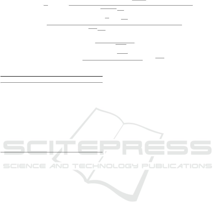
As in (Nasir and Guo, 2019) and (Meng and
Chen, 2020), we define for each AP-UE link an agent,
thus the power allocation is performed by a multi-
agent system, where each agent contains a DQN. The
agents interact with the environment to collect data
(s
t
,a
t
,r
t
,s
t+1
) and store it in a dataset at the CC, then
by mini-batch sampling the DQN is trained using the
gradient descent algorithm, as shown in Fig.3. Since
the learning is done off-line, the overhead cost of the
data collection does not affect the operational phase.
It is unnecessary to have ‘real-time’ training in off-
line learning mode. The training time, however, could
be considerable. We also should clarify that for the
off-line learning mode, the DQN is trained by a suffi-
cient dataset, the size depends on the convergence of
the sum-SE. Once the training is finished, the DQN
is used to perform the power allocation. No further
training is needed. However, when there are signif-
icant changes in the network configuration, e.g., the
number of active APs, or in the temporal and spatial
traffic characteristics, the DQN should be retrained.
When that should happen and what impact it would
have on the operation of the system has not been ad-
dressed yet and requires further study.
There is a total of NK agents in the whole system.
At time step t, each agent (n,k) allocates power from
AP n to UE k. One should note that all agents use the
same DQN parameters, i.e., after the DQN is trained
by the experience of all agents, the DQN shares its
parameters with all other agents to allocate power.
We define e
t
n,k
= (s
t
n,k
,a
t
n,k
,r
t
n,k
,s
t+1
n,k
) as the experi-
ence sequence of agent (n,k) at time step t. The DQN
is trained by the dataset D = {e
1
1,1
,e
1
1,2
,. . . ,e
t
n,k
. . . },
which describes the agents’ relation with their envi-
ronment. The key to using the DQN for solving (5)
is to model the decision variables as the action of
agents. Obviouly the normalized downlink transmis-
sion power p
n,k
is the decision variable for SE, there-
fore the action of agent (n,k) is p
n,k
. We define p
t
n,k
as
the action of agent (n,k) at time step t. The agent (n,k)
takes action according to the current state s
t
n,k
, which
features the independent variables. From (4) we find
that the large-scale fading is the independent variable
for SE, therefore the large-scale fading matrix at time
step t,
β
β
β
t
=
β
t
1,1
β
t
1,2
... β
t
1,K
β
t
2,1
β
t
2,2
... β
t
2,K
... ... ... ...
β
t
N,1
β
t
N,2
... β
t
N,K
(14)
is a key element for s
t
n,k
. The objective function,
which describes the target of the agents, is defined
as the reward, i.e., the downlink sum-SE, achieved in
each time step. Based on the above analysis, the el-
ements of the experience etnk for CF mmWave mas-
sive MIMO power allocation are defined as following:
1) State s
t
n,k
: The signal-to-interference-plus-
noise ratio (SINR) is the key element of the SE.
The signal in SINR of UE k comes from the agent
set {(1,k), (2,k),. . . ,(N,k)}, while the interference in
SINR for agent (n, k) mainly comes from the agent
set {(n,1), (n,2),. . . ,( n,K)}. Therefore, for agent (n,
WINSYS 2021 - 18th International Conference on Wireless Networks and Mobile Systems
38
link (n,k)
UE k
AP n
Environment
Reward
Action
State
Agent(n,k)
State
DQN
Parameter θ
Policy
π(s,a)
2. Interaction with environment
3. Dataset
Parameters
4. Training
1. Initialization
Design of the DQN
and parameter selection
UE k-1
AP n-1
link (n,k-1)
Record
Sampling
link (n-1,k-1)
link (n-1,k)
5. Testing
Parameters
e
t
nk
=(s
nk
t
, a
nk
t
, r
nk
t
, s
nk
t+1
)
D={e
1
11
, e
1
12
,… e
t
NK
}
Mini-batch
Gradient
descent
New
parameters
Performance and
execution time
Figure 3: Illustration of the proposed multi-agent deep reinforcement learning system.
k) only the n-th row and k-th column of β
β
β
t
are rel-
evant. We normalize these elements by β
t
n,k
as data
preprocessing. It has been determined experimentally
that some auxiliary information can improve the sum-
SE performance of DQN. Like in (Nasir and Guo,
2019) and (Meng and Chen, 2020), we consider two
auxiliary information elements, namely the sum-SE
∑
K
k
0
=1
SE
t−1
k
0
and the power allocation p
t−1
n,k
at time step
t-1. Finally, s
t
n,k
is formalized as follows:
s
t
n,k
= {
β
β
β
t
(n,:)
β
t
n,k
,
β
β
β
t
(:,k)
/β
t
n,k
β
t
n,k
, p
t−1
n,k
,
K
∑
k
0
=1
SE
t−1
k
0
} (15)
where β
β
β
t
(n,:), β
β
β
t
(:,k) represent the n-th row and k-th
column of β
β
β
t
, respectively. The numerator of the sec-
ond term in s
t
n,k
removes a redundant β
t
n,k
. Therefore
the size of s
t
n,k
, i.e., the input dimension of the DQN,
is N + K + 1. One remark is that
∑
K
k
0
=1
SE
t−1
k
0
in (15)
is the sum-SE at time step t −1. Each UE measures
its SE and then sends it to the APs by the uplink at
time step t −1. Then the CC collects this information
as the input of the DQN at time step t. The process
of sending SE values can be neglected in the power
allocation process, since it occurs on the time scale of
large-scale fading, similar to the β
β
β
t
collection. In ad-
dition, compared to the β
β
β
t
matrix (KNelements), there
are only K elements of the SE information i.e., the SE
of K UEs.
2) Action a
t
n,k
: The allocated power is a continu-
ous variable, however, for the action space of DQN,
the dimension must be finite. Therefore we discretize
the power as follows:
A
A
A = {0,
p
max
|A
A
A|−1
,
2p
max
|A
A
A|−1
,..., p
max
} (16)
where |A
A
A| represents the number of power levels.
3) Reward r
t
n,k
: The target is to maximize the sum-
SE. Therefore, the reward is the sum-SE at time step
t:
r
t
n,k
=
K
∑
k=1
SE
t
k
(17)
3.3 Complexity of the Proposed DQN
The computational complexity considers the opera-
tional phase, i.e., the time period that a trained DQN
performs the power allocation. Therefore the com-
putational complexity of the DQN is only determined
by the DNN. The computational complexity of a neu-
ral network depends on the number of neurons and
layers. Specifically, for a fully-connected neural net-
work, the complexity is O(νµ
2
), where ν is the num-
ber of layers and µ is the number of neurons for
the widest layer, i.e., the layer with the most neu-
rons. Typically, the number of neurons in each layer
depends on the dimension of the input layer, i.e.,
O(µ)=O(N +K + 1) in our case. The number of layers
for a DQN is independent of the scale of the problem.
Therefore the computational complexity of DQN is
Deep Reinforcement Learning for Dynamic Power Allocation in Cell-free mmWave Massive MIMO
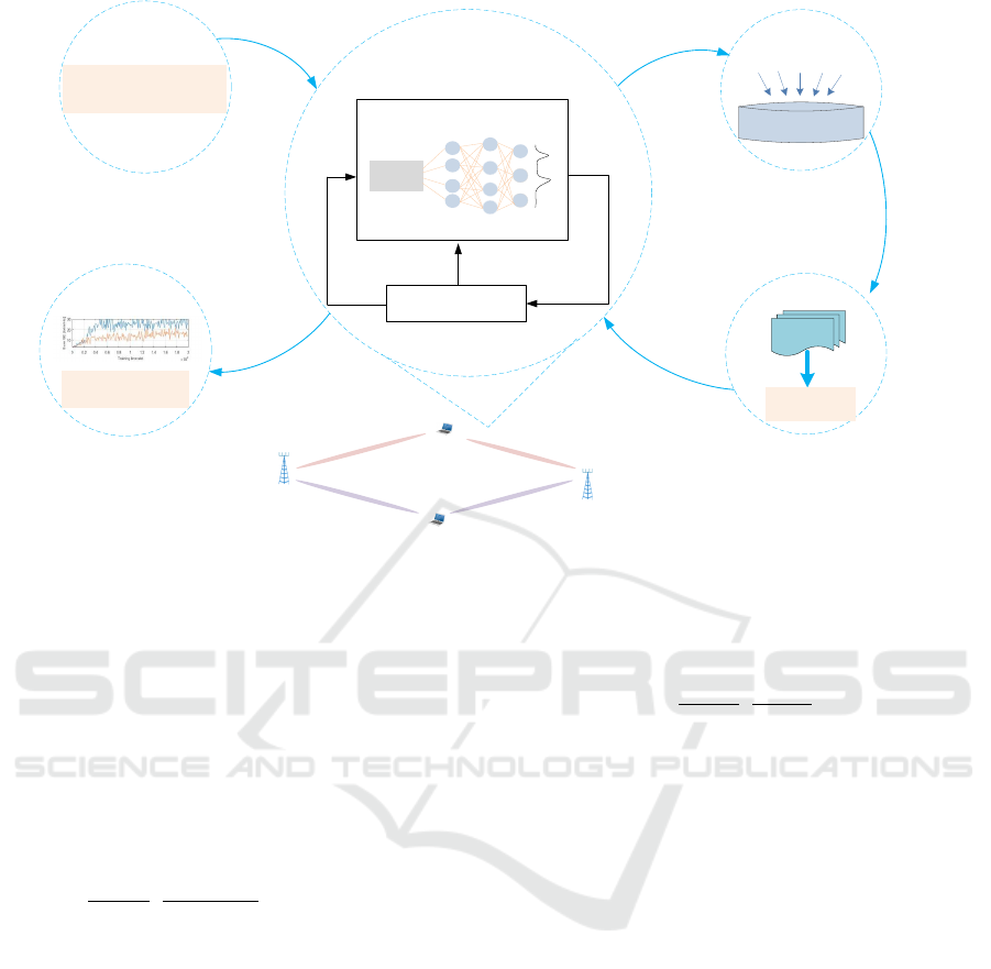
39
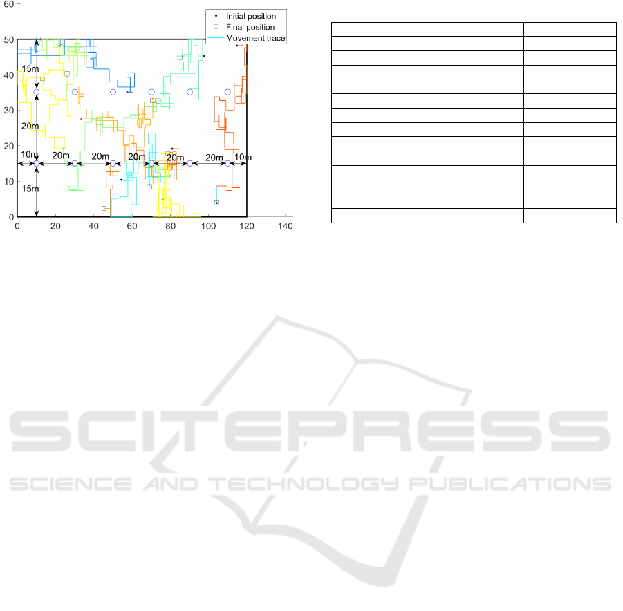
Figure 4: Example of UE movement traces in a 3GPP TR
38.901 scenario for 100 seconds.
O(N
2
+ K
2
). Compared to the WMMSE algorithm
O(IN
2
K
3
) in Section 2.4, the DQN has a much lower
computational complexity.
4 SIMULATION RESULTS
In this section we show by simulations that the
DQN-based power allocation in CF mmWave mas-
sive MIMO is competitive in terms of performance
and complexity.
4.1 Scenario and Configuration
We consider the 3GPP TR 38.901 indoor mixed of-
fice scenario (120m×50m×3m) (3GPP, 2018) with
12 APs. Each AP contains 9 antennas in a horizon-
tally mounted and downward radiating 3×3 UPA at a
height of 3m. We assume K=10 single-antenna UEs
moving within the coverage area. Each UE moves in
a random direction (up, down, left, and right) with
a randomly chosen velocity distributed uniformly be-
tween 0 and 1m/s. We consider a discrete time system
where the duration of each time step is 0.2s, corre-
sponding to the large-scale time (40 coherence times),
as discussed in Section 3.2. The carrier frequency is
29 GHz, the bandwidth is 200 MHz. For a UE ve-
locity of 1m/s, the channel coherence τ
c
is about 5
ms, calculated as τ
c
= λ/2v, where λ is the wave-
length and v is the velocity (Marzetta and Ngo.H.Q,
2016). Each UE maintains its speed and direction in
each second before selecting a new speed and direc-
tion. The initial positions of the UEs at time t=0, are
uniformly distributed over the coverage area (Fig.4).
We model the large-scale fading as the combination
of pathloss and shadowing, as in (3GPP, 2018).
Table 1: Parameters used in simulations.
Parameter value
Coverage volume 120m×50m×3m
K, number of UEs 10
M, number of antennas per AP 9
N, number of APs 12
p
max
, maximum power constraint 13 dBm
p
p
, pilot power 20 dBm
τ
c
, length of coherence time in symbols 200
τ
p
, length of pilot in symbols 5
Carrier frequency 29 GHz
Bandwidth 200 MHz
Noise power -74dBm
Distribution of UE velocity U(0, 1) m/s
Timeslot duration 0.2s
The maximum power constraint p
max
is 13 dBm
and the noise power is assumed to be -74 dBm. The
uplink pilot power is 20 dBm. We set the coher-
ence time to 200 modulation symbols as in (Q and
Ashikhmin, 2017). We assume the length of the up-
link pilot, used to determine the CSI, is 5 symbols. As
discussed in (Q and Ashikhmin, 2017), when τ
p
< K
some pilot sequences are reused, hence the simula-
tions take pilot contamination into consideration. The
parameters used in the simulations are listed in Table
I.
4.2 DQN Parameter Selection
We adopted a four-layer fully connected neural net-
work, where the number of neurons in the two hid-
den layers are 128 and 64, respectively. This choice
was based on what was proposed and worked well in
(Nasir and Guo, 2019) and (Meng and Chen, 2020).
We did not investigate whether different values for
these hyperparameters would lead to better results.
This may be a topic for further study. The number of
neurons in the input layer is N +K + 1 as discussed in
(20), i.e., 22 in our case. We set the number of power
levels equal to 10; therefore, the number of neurons
in the output layer is 10.
It is worth pointing out that finding the best DQN
parameters can be seen as an optimization problem
in its own right. For a given problem, the training
should be based on the particular network configura-
tion and the usage scenarios to be expected. In this
subsection we tried several parameters to find the best
choice, i.e., those that give us the highest sum-SE dur-
ing training. We studied the impact of the discount
factor ω, the training interval C, the initial adaptive
learning rate lr and the adaptive ε-greedy algorithm
on the training of the DQN.
Adaptive learning means that the learning rate
WINSYS 2021 - 18th International Conference on Wireless Networks and Mobile Systems
40

decays with the number of training time steps. Gen-
erally, a large learning rate allows the model to learn
faster but may end up with a sub-optimal final set of
weights. A smaller learning rate may allow the model
to learn a more optimal or even globally optimal
set of weights but may take significantly longer.
Adaptive learning balances the training time and
performance. The ε-greedy algorithm is a learning
method that makes use of the exploration-exploitation
tradeoff, in which the agent takes a random action
(choosing a power level) with probability ε or takes
the DQN output with probability 1-ε. A random
action may lead the training ‘jumps’ out of a local
optimum and explores new convergence regions.
In the adaptive ε-greedy algorithm the value of ε
decays each training time step. A large ε avoids
the training ending up in local optima during the
intial training time steps, a small value of ε makes
sure that the training will converge in the later
training time steps. Referring to the literatures,
we choose ω ∈ {0.1,0.3,0.5,0.7, 0.9}(Meng.F
and P., 2019), C ∈ {10,50,100, 200,500}(Nasir
and Guo, 2019; Mnih and Kavukcuoglu,
2013), lr ∈ {0.001,0.005, 0.01,0.05,0.1}(Chien
and Canh, 2020; Nasir and Guo, 2019),
ε ∈ {0.1,0.3,0.5, 0.7,0.9}(Mnih and Kavukcuoglu,
2013; Meng.F and P., 2019) to find the optimal
configurations.
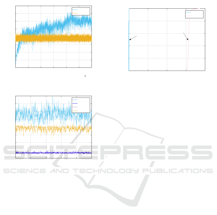
Fig.5 shows the effect of different parameters on
the training process. The graphs on the left show the
sum-SE as a function of time over a period of 20000
time steps. The corresponding graphs on the right
show the empirical CDF of the sum-SE. In each of
the figures we vary one parameter, while keeping the
others constant.
Fig.5(a) shows the effect of the discount factor ω.
Although the differences are not pronounced, we see
that the sum-SE for ω=0.1 is always larger than for
ω=0.9, by observing that the red line is to the right
of the the blue line in the empirical CDF graph. The
fluctuations of the sum-SE as a function of the train-
ing time, is due to the random mobility of the UEs,
which leads to a variation of the large-scale fading.
Fig.5 (b) shows the effect of the training interval
C. Similar observations can be found as in Fig.5(a),
the differences between the lines are not pronounced.
Nevertheless we find that C=100 achieves the highest
sum-SE, by observing the light blue line in the empir-
ical CDF graph.
Fig.5(c) shows the effect of the initial learning rate
lr. The differences between the lines are not obvious,
but we still see that the sum-SE for lr=0.005 achieves
the highest sum-SE, by observing the light red line is
to the right of other lines in the empirical CDF graph.
Fig. 5(d) shows the effect of ε-algortihm. We find
that for different values of ε, the values of sum-SE
are very different. It is obvious that ε=0.1 achieves
the highest sum-SE, by observing the red line in both
training process and empirical CDF graphs.
Based on the above observations, we choose the
parameters ω=0.1, C=100, lr=0.005 and ε=0.1 to train
the DQN. The length of the training period we choose
is determined by the time it takes for the time-average
of the sum-SE to converge to a stable value, i.e., a
longer training period does not result in a significantly
different time-average. In our case 30000 time steps,
appears to be sufficiently long, as can be observed
from Fig.6.
Observe that DQN achieves sum-SE values fluctu-
ating around 23 bit/s/Hz around 5,000th training time
steps. Afterward the average rises slowly and finally
converges to around 30 bit/s/Hz after 20,000 training
time steps. This is obviously better than the value
obtained by the WMMSE algorithm, which is also
shown in the figure as a reference benchmark. The
random mobility of UEs causes the fluctuations of the
sum-SE for both methods. It is clear that the DQN
method, after sufficient training, achieves signifi-
cantly better average sum-SE values than WMMSE.
4.3 Sum-SE Performance
We have used three benchmark algorithms to evalu-
ate the performance of the DNQ based-power alloca-
tion. The first benchmark is the WMMSE algorithm
described in Section 2.4, which is well-adopted and
has been shown to perform well in cases studied in
the literature (Sun and Chen, 2018; Nasir and Guo,
2019; Meng.F and P., 2019). The second benchmark
is random power allocation where p
n,k
∼U(0, p
max
)
for all n and k. The third one is full power allocation,
i.e.,p
n,k
= p
max
for all n and k. We use the DQN that
has been trained for 30000 time steps, as described
in Fig.6 and run it for 1000 time steps. Fig.7 shows
the sum-SE of the four methods over a period of 1000
time steps.
As expected, WMMSE and DQN have much bet-
ter performance than random and full power alloca-
tion. In addition, the DQN method performs sig-
nificantly better than WMMSE. The DQN method
achieves around 10 bit/s/Hz higher sum-SE than the
WMMSE algorithm.
4.4 Computational Complexity
Comparison
To get an indication of the difference in computational
complexity of DQN and WMMSE, we measured the
Deep Reinforcement Learning for Dynamic Power Allocation in Cell-free mmWave Massive MIMO
41
0 0.5 1 1.5 2
Training time step
10
4
0
5
10
15
20
25
30
Sum SE [bit/s/Hz]
=0.1
=0.3
=0.5
=0.7
=0.9
0 10 20 30 40
Sum SE[bit/s/Hz]
0
0.2
0.4
0.6
0.8
1
F(x)
Empirical CDF
=0.1
=0.3
=0.5
=0.7
=0.9
(a) Discount factor ω selection with training interval C = 10, initial learning rate lr = 0.001, ε = 0.1.
0 0.5 1 1.5 2
Training time step
10
4
5
10
15
20
25
30
Sum SE [bit/s/Hz]
C=10
C=20
C=50
C=100
C=200
0 10 20 30 40
Sum SE[bit/s/Hz]
0
0.2
0.4
0.6
0.8
1
F(x)
Empirical CDF
C=10
C=20
C=50
C=100
C=200
(b) Training interval C selection with discount factor ω = 0.1, initial learning rate lr = 0.001, ε = 0.1.
0 0.5 1 1.5 2
Training time step
10
4
5
10
15
20
25
30
Sum SE [bit/s/Hz]
lr=0.001
lr=0.005
lr=0.01
lr=0.05
lr=0.1
0 10 20 30 40
Sum SE[bit/s/Hz]
0
0.2
0.4
0.6
0.8
1
F(x)
Empirical CDF
lr=0.001
lr=0.005
lr=0.01
lr=0.05
lr=0.1
(c) Initial learning rate lr selection with discount factor ω = 0.1, training interval C=10, ε = 0.1.
0 0.5 1 1.5 2
Training time step
10
4
5
10
15
20
25
30
Sum SE [bit/s/Hz]
=0.1
=0.3
=0.5
=0.7
=0.9
0 5 10 15 20 25 30 35
Sum SE[bit/s/Hz]
0
0.2
0.4
0.6
0.8
1
F(x)
Empirical CDF
=0.1
=0.3
=0.5
=0.7
=0.9
(d) ε selection with discount factor ω = 0.1, training interval C=10, initial learning rate lr = 0.001.
Figure 5: Effect of different parameters on the training process.
WINSYS 2021 - 18th International Conference on Wireless Networks and Mobile Systems
42
0 0.5 1 1.5 2 2.5 3
Training time step
10
4
0
5
10
15
20
25
30
35
40
Sum SE [bit/s/Hz]
DQN
WMMSE
Figure 6: Training process of DQN with ω = 0.1,C =
100,lr = 0.005,ε = 0.1.
0 200 400 600 800 1000
Time slot
0
5
10
15
20
25
30
35
40
Sum SE[bit/s/Hz]
DQN
Full
Random
WMMSE
Figure 7: Comparison of sum-SE of DQN with the bench-
mark power allocation schemes over 1000 time steps, where
DQN is trained with ω = 0.1,C = 100, lr = 0.005, ε = 0.1.
execution time in each of the 1000 time steps. We ran
the algorithms on a 4 core Intel Core i5-7300 CPU
with 2.6 GHz frequency. The programs are coded in
Python 3.7.2 (DQN with Tensorflow 1.13.1). Fig.8
shows the empirical CDF of the execution times that
we recorded for the two methods.
From Fig.8 it is obvious that DQN requires much
less processing time than WMMSE and has less varia-
tion. It is around 0.6 ms for DQN while for WMMSE
the execution time ranges from 600 ms to 750 ms.
Recall that the power allocation is performed within
each large-scale time, namely 0.2s in our case. It is
obvious the DQN method meet this time constraint,
while the WMMSE does not.
In addition, for DQN, the number of calculations
is constant, as the number of neurons and layers does
not change. Although it is invisible in Fig.8, there
are still some slight fluctuations of execution time,
which come from the calculation of different floating-
point numbers and the inaccuracy of reading the sys-
tem time. For WMMSE, the time fluctuation mainly
0 200 400 600 800
Execution time[ms]
0
0.2
0.4
0.6
0.8
1
F(x)
Empirical CDF
DQN
WMMSE
The median:626.8
The median:0.63
Figure 8: Execution time for DQN and WMMSE.
comes from different initializations, i.e., a different
initial point of the algorithm can make a large dif-
ference in the time needed to find the optimum. So
we can conclude that the DQN method is expected to
meet the requirements of real-time power allocation
in a real implementation. One should note that the ex-
ecution times shown in Fig.8 do not take into account
the overhead for the information exchange between
the APs and the CC via the fronthaul.
5 CONCLUSION
In this paper, we studied the use of DQN to allo-
cate transmission power for maximizing the down-
link sum-SE in CF mmWave massive MIMO systems
with mobile UEs in an indoor scenario. Imperfect CSI
and uplink pilot contamination were considered in the
analysis. Unlike supervised learning that needs a huge
dataset generated by other algorithms, the DQN is
trained by interacting with the environment. The ob-
jective function, i.e., the sum-SE, is used as the re-
ward to train the DQN. The sum-SE obtained by the
DQN is significantly higher than the one achieved by
the well-adopted WMMSE algorithm. In addition, the
time-complexity of the DQN method is very low. The
numerical results show that the DQN is expected to
satisfy the stringent time constraints of power alloca-
tion in CF mmWave massive MIMO. There are still
open issues to be addressed:
1. Online learning, which is expected to be pro-
cessed in the real deployment of DQN, should be fur-
ther studied to accommodate the scenarios with real
measurements of channels and mobility of real UEs.
2. Different power allocation objective function,
e.g., max-min policy, should be studied.
3. We assumed a Markovian UE mobility model.
The mobility of real UEs is non-Markovian, which
Deep Reinforcement Learning for Dynamic Power Allocation in Cell-free mmWave Massive MIMO
43

might lead to an inefficient training of the DQN. This
should be further investigated.
4. When, during operation, significant changes in
the network configuration, e.g., the number of active
APs, or in the temporal and spatial traffic characteris-
tics, occur, the DQN should be retrained. When that
should happen and what impact it would have on the
operation of the system has not been addressed yet
and requires further study.
5. For the hyper-parameters of the DQN, i.e., the
number of layers and neurons, we used values taken
from the literature. One could investigate whether
these hyper parameters could be optimized to get bet-
ter results in terms of the achieved sum-SE.
REFERENCES
3GPP (2018). Study on channel model for frequencies from
0.5 to 100 GHz (Release 15). In IEEE 21st Interna-
tional Workshop on Computer Aided Modelling and
Design of Communication Links and Networks. 3GPP.
Alkhateeb, A. and Mo, J. (2014). MIMO precoding and
combining solutions for millimeter-wave systems. In
IEEE Communications Magazine. IEEE.
Alonzo, M. and Buzzi, S. (2019). Energy-efficient power
control in cell-free and user-centric massive MIMO
at millimeter wave. In IEEE Transactions on Green
Communications and Networking. IEEE.
Andrews and G., J. (2014). What will 5G be? In IEEE
Journal on Selected Areas in Communications. IEEE.
Bj
¨
ornson, E. and Hoydis, J. (2017). Massive MIMO
Networks: Spectral, Energy, and Hardware Effi-
ciency. Foundations and Trends in Signal Processing,
Hanover.
Busari, S. A. and Huq, K. M. S. (2018). Millimeter-wave
massive MIMO communication for future wireless
systems: A survey. In IEEE Communications Surveys
& Tutorials. IEEE.
C, G. and K, H. (2013). On mm-wave multipath cluster-
ing and channel modeling. In IEEE Transactions on
Antennas and Propagation. IEEE.
Chen, Z. and Bj
¨
ornson, E. (2018). Channel hardening
and favorable propagation in cell-free massive MIMO
with stochastic geometry. In IEEE Transactions on
Communications. IEEE.
Chien, T. V. and Canh, T. N. (2020). Power control in cellu-
lar massive MIMO with varying user activity: A deep
learning solution. In IEEE Transactions on Wireless
Communications. IEEE.
F, S. and W., Y. (2016). Hybrid digital and analog beam-
forming design for large-scale antenna arrays. In
IEEE Journal of Selected Topics in Signal Processing.
IEEE.
Gonz
´
alez-Coma, J. P. and Rodr
´
ıguez-Fern
´
andez, J. (2018).
Channel estimation and hybrid precoding for fre-
quency selective multiuser mmWave MIMO systems.
In IEEE Journal of Selected Topics in Signal Process-
ing. IEEE.
Hamdi, R. and Driouch, E. (2016). Resource allocation in
downlink large-scale MIMO systems. In IEEE Access.
IEEE.
I, A. and H, K. (2018). A survey on hybrid beamforming
techniques in 5G: Architecture and system model per-
spectives. In IEEE Communications Surveys & Tuto-
rials. IEEE.
Interdonato, G. and Ngo, H. Q. (2016). On the performance
of cell-free massive MIMO with short-term power
constraints. In IEEE 21st International Workshop on
Computer Aided Modelling and Design of Communi-
cation Links and Networks. IEEE.
Larsson, E. G. and Edfors, O. (2014). Massive MIMO for
next generation wireless systems. In IEEE Communi-
cations Magazine. IEEE.
LeCun and Bengio (2015). Deep learning. In Nature. Na-
ture.
Lin and Cong, J. (2019). Hybrid beamforming for millime-
ter wave systems using the MMSE criterion. In IEEE
Transactions on Communications. IEEE.
M, L. and T., Z. (2014). Efficient mini-batch training for
stochastic optimization. In Proceedings of the 20th
ACM SIGKDD international conference on Knowl-
edge discovery and data mining. ACM.
Mai, T. C. and Ngo, H. Q. (2020). Downlink spectral
efficiency of cell-free massive MIMO systems with
multi-antenna users. In IEEE Transactions on Com-
munications. IEEE.
Marzetta and Ngo.H.Q (2016). Fundamentals of massive
MIMO. Cambridge University Press, Cambridge.
Meng, F. and Chen, P. (2020). Power allocation in multi-
user cellular networks: Deep reinforcement learning
approaches. In IEEE Transactions on Wireless Com-
munications. IEEE.
Meng.F and P., C. (2019). Power allocation in multi-user
cellular networks with deep Q learning approach. In
IEEE International Conference on Communications.
IEEE.
Mnih and Kavukcuoglu (2013). Human-level control
through deep reinforcement learning. In Nature. Na-
ture.
N, B. E. and H, I. (1989). The Bellman equation for min-
imizing the maximum cost. In Nonlinear Analysis:
Theory, Methods & Applications.
Nasir, Y. S. and Guo, D. (2019). Multi-agent deep rein-
forcement learning for dynamic power allocation in
wireless networks. In IEEE Journal on Selected Ar-
eas in Communications. IEEE.
Nikbakht, R. and Jonsson, A. (2019). Unsupervised-
learning power control for cell-free wireless systems.
In IEEE 30th Annual International Symposium on
Personal, Indoor and Mobile Radio Communications.
IEEE.
O., E. A. and S., R. (2014). Spatially sparse precoding in
millimeter wave MIMO systems. In IEEE transac-
tions on wireless communications. IEEE.
Polegre, A. . and Palou, F. R. (2020). New insights on chan-
nel hardening in cell-free massive MIMO networks. In
WINSYS 2021 - 18th International Conference on Wireless Networks and Mobile Systems
44

2020 IEEE International Conference on Communica-
tions Workshops. IEEE.
Q, N. H. and Ashikhmin (2017). Cell-free massive MIMO
versus small cells. In IEEE Transactions on Wireless
Communications. IEEE.
Shi, Q. and Razaviyayn, M. (2011). An iteratively weighted
MMSE approach to distributed sum-utility maximiza-
tion for a MIMO interfering broadcast channel. In
IEEE Transactions on Signal Processing. IEEE.
Sun, H. and Chen, X. (2018). Learning to optimize: Train-
ing deep neural networks for interference manage-
ment. In IEEE Transactions on Signal Processing.
IEEE.
Yu, X. and Shen, J. (2016). Alternating minimization al-
gorithms for hybrid precoding in millimeter Wave
MIMO systems. In IEEE Journal of Selected Topics
in Signal Processing. IEEE.
Deep Reinforcement Learning for Dynamic Power Allocation in Cell-free mmWave Massive MIMO
45
