
Agent-based Intelligent KPIs Optimization of Public Transit Control
System
Nabil Morri
1,3 a
, Sameh Hadouaj
2,3 b
and Lamjed Ben Said
3c
1
IT Department, Emirates College of Technology, Abu Dhabi, U.A.E.
2
Computer Information Systems Department, Higher Colleges of Technology, U.A.E.
3
SMART Lab., Institut Supérieur de Gestion de Tunis, Université de Tunis, Tunisia
Keywords: Public Transit, Intelligent Control System, Optimization, Multi-agent System, Key Performance Indicator.
Abstract: Public transit has a wide variety of resources. There is an infrastructure including stations and routes with
multiple trips provided by different modes of transportation (metro, subway, bus). These resources must be
well exploited to ensure good quality of service to passengers and especially against perturbations that may
occur during the day. The contribution of this work is to model and implement a transit control system that
detects perturbations and finds, through optimization, the best regulation action while respecting the
constraints of the traffic situation. This system combines various measures of Key Performance Indicators
(KPIs) into a single performance value, covering several dimensions depending on the type of service quality
to be guaranteed. To take into account the complex and dynamic nature of transportation systems, a multi-
agent approach is adopted in the modelling of our system. The validation is based on real traffic data. The
results show better performance of our system compared to the current resolution.
1 INTRODUCTION
Today, public transportation is one of the most
important elements of the municipal plan. In densely
populated urban areas, it carries a large number of
people and becomes an indispensable service in daily
life. In addition, public transport networks have been
expanded. The number of vehicles, stations and
itineraries continues to grow. This makes the
management challenges even more complex.
With the emergence of many complex and
random phenomena that disrupt transit traffic, it is
becoming difficult to keep up with scheduled vehicle
timetable in real time. For that reason, the quality of
public transit service is deteriorating. Furthermore,
the complexity of the road network means that several
perturbations can occur at the same time and that one
perturbation can generate others.
In addition, the transit system must be able to
adapt to changing traffic conditions to ensure the
required quality of service. They must therefore
detect disturbances quickly and deal with new
situations in order to improve the quality of service
a
https://orcid.org/0000-0002-1642-9309
b
https://orcid.org/0000-0002-6743-4036
c
https://orcid.org/0000-0001-9225-884X
through performance measures. These measures are
known as KPIs, which are quantitative measures or
indices that numerically express a specific quality.
There is an extensive literature on various aspects
of KPIs. (Mark Tromp et al., 2011) evaluates
performance by EWT: Excess Wait Time, AWT:
Actual Wait Time and SWT: Scheduled Wait Time.
Moreover, in (M. Napiah et al., 2015) this performance
is defined by the average waiting time expected by
passengers. (Oded Cats et al., 2010) defines
performance by the observed time interval deviations
between trips of the same line compared to the regular
frequency of vehicles during a given period.
(Neila Bhouri et al., 2016) describes the Gini
index as another indicator in the form of a forward
regularity index. (S. Carosi a, et al., 2015) describes
regularity as an index on vehicle entries at stations.
Other projects define another indicator which is
punctuality as a determining criterion in the final
performance formulation. Punctuality is defined in
(Noorfakhriah Y. and Madzlan N., 2011) as a
comparison of actual departure times and scheduled
departure times at the station. In (Xumei Chen et al.,
224
Morri, N., Hadouaj, S. and Ben Said, L.
Agent-based Intelligent KPIs Optimization of Public Transit Control System.
DOI: 10.5220/0010616302240231
In Proceedings of the 18th International Conference on Informatics in Control, Automation and Robotics (ICINCO 2021), pages 224-231
ISBN: 978-989-758-522-7
Copyright
c
2021 by SCITEPRESS – Science and Technology Publications, Lda. All r ights reserved
2009) the authors distinguish three measures of
punctuality. PIR: Punctuality Index based on Routes,
DIS: Deviation Index based on Stops and EIS:
Evenness Index based on Stops. However, in
(Vaniyapurackal, 2015), the author converts the
punctuality index to a percentage to define the
proportion of the trip that was punctual.
In (Saberi, Meead, et al., 2012), three alternative
performance measures are proposed: EI: Earliness
Index, WI: Width Index and SSD: Second-Order
Stochastic Dominance Index. These indices are used
in two forms to measure the unreliability of a bus
service: (i) the distribution of lane deviations for
frequent services and (ii) the distribution of delays for
infrequent services.
Other work, such as of (Ceder, 2007), add another
indicator called transfer time that covers the time
spent when the passenger is waiting for the vehicle
while changing the line at a transfer station.
(Zhenliang, 2013) details and explains the Input
Buffer Time (IBT) formula that can be used to
understand the additional unreliability caused by an
incident. The authors of (Kenneth et al., 2004) and
(Levinson, Herbert, 1983) discuss another indicator
called "Dwell"" which is the parking time of vehicles.
"Dwell" can also be used to hold for traffic to be
restored (Vu The Tran et al., 2012) (Cats et al., 2011).
From this literature, we note that there is no
standard meaning for specifying and formulating
performance indicators. The challenge in defining
key performance indicators is to select those that will
sufficiently satisfy the overall performance of public
transport.
In addition, the task of transit control is based on
the optimization of the KPIs. The transit system must
provide comparative information that allows the
control system to identify performance gaps and set
measures and targets to resolve them.
Multi-agent modelling can provide a solution
fitted to the activities of public transport networks
where autonomous entities (buses, stations,
itineraries, etc.), called agents, dispersed in a dynamic
environment which is the traffic of the transport
network. They adapt their behaviours to the
perturbation they perceive and interact with each
other to perform optimal regulation actions.
Our objective is to model and implement an
intelligent control system that manages perturbations.
It detects and finds the best regulation action while
respecting the constraints of the traffic situation. This
system combines various KPI measures into a single
performance value, covering several dimensions
depending on the type of service quality to be
guaranteed.
This paper is organized as follows. Section 2
defines the perturbation and describes the control
method. Section 3 presents the performance
measures. Section 4 details mathematical model by
formulating the optimization problem. Section 5
presents the multi-agent model by describing the
agents with their behaviours. Section 6 validates the
control strategy of our system on a real network in the
city of Portland in Oregon. In Section 7, we conclude
and provide some perspectives.
2 PERTURBATION AND
CONTROL METHOD
2.1 Perturbation
In general, a perturbation is the unexpected, sudden,
or progressive appearance of events that can modify
or cancel a program. In the field of public transport, a
perturbation is an event that appears suddenly
modifying the traffic state of the network in a
situation that is generally unsatisfactory in terms of
service quality. The perturbation then affects the
normal operation of the network, which consists of
keeping the scheduled timetable of vehicles.
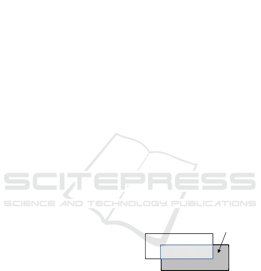
Therefore, to improve service performance, it is
necessary to optimize the adequacy between
scheduled and actual operations as shown in Figure 1.
In his study, (Van Oort, 2009) values the perturbation
as guidelines to control the variation of scheduled
operations from actual.
Figure 1: Inadequacy between scheduled and actual
operations.
2.2 Control Method
(Ashby, W.R., 1956) presents three main methods of
general control. These control methods are designed
to mitigate the negative effects of perturbations on the
process and allow to achieve the desired results.
Use of a Buffer: consists in providing resources
in the form of a measurement buffer allowing
to detect the perturbation without generating
repercussions on the desired result;
Actual operations
Scheduled operations
Adequacy
The process
variation
Agent-based Intelligent KPIs Optimization of Public Transit Control System
225
Feedback: In case of unacceptable variation
between scheduled and actual operations, a
regulator intervenes to restore the desirable
situation;
Feed-forward: Instead of observing the trends
of the variation, the regulator prepares the
regulation action based on the simulation.
The three methods have specific advantages and
disadvantages. In practice, they can also be used in
combination. In our study, the control method is
mainly used to evaluate current performance and to
adjust operations in case of inadequate performance.
Therefore, it is essential to have the resources for
detecting the perturbation and a regulator to reduce
the variation as much as possible. Consequently, in
our model it is necessary to have a buffer for the
detection. While, after detection the selection of the
control action is based on the calculation of the
performance measurements of several regulation
maneuvers. This is the feedback method.
As well, it is necessary to have scenarios of
control maneuvers in memory to be able to compare
the predicted results with the results of the scenarios.
This is the feed-forward method.
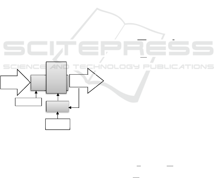
Therefore, the three control methods that are
mentioned above are used in combination in the
modelling of our control system. We describe in the
figure 2 the control method used in our modelling.
Figure 2: Control method of our system.
3 THE PERFORMANCE
MEASURES
3.1 Selected Traffic Performance
Indicators
The list of selected KPIs that measure performance
quality are based on the indices of the "operational
efficiency" objective. According to literature reviews
by (Cambridge Systematics Inc. 2005), this objective
will be focused on three indicators: punctuality,
regularity, and correspondence. The other indicators
that are related to the costs of transport, such as oil
consumption and the number of kilometers traveled,
are not included in our study, because our control
system is oriented towards the user of the transport
system and not the operator, and they are irrelevant
for the passengers.
The formulas for these measures are taken from
(European Commission, 2011) and some other
research works such as (Yan et al., 2009),
(Noorfakhriah Y. and Madzlan N., 2011) and (Ceder,
2007). They represent a standard that can evaluate
overall traffic performance in transportation
engineering and Intelligent Transportation Systems.
3.2 Punctuality Index
Punctuality is defined in (Noorfakhriah Y. and
Madzlan N, 2011) (Saberi, Meead, et al, 2013) as a
comparison between the actual and the scheduled
arrival times at the station. Its formula is:
I
=
avec S
=
∑
(t
−t
)
(1)
n: the number of vehicles.
PUN
:
∑
(PUN
−PUN
)
the average
punctuality for the n vehicles.
t
=t
_
+Dwel
: the actual departure time
of the i-th vehicle, while Dwel
is the time
spent board the passengers.
Dwel
= t
∗ N
− t
∗ N
,
with t
et t
are the average time spent
by the passenger to get on or off the vehicle and
N
et N
are the number of passengers to
be picked up and dropped off the vehicle.
t
: the scheduled departure time.
3.3 Regularity Index
The regularity index measures the differences in time
intervals observed at the station between successive
vehicles of the same line compared to the scheduled
frequencies. The formula of the regularity index is:
I
=
avec S
=
∑
(h
−h
)
(2)
h
:
∑
(t
−t
)
the average frequency
for the n vehicles.
h
i
: t
i
– t
i-1
(i=2,…I), the current time interval.
h
: the scheduled time interval.
Data: Curren
t
state of traffic
Process
Current results
and maneuvers
Perturbations
Regulator
Regulation
Buffer:
detector,
sensor,
camera,
GPS...
ICINCO 2021 - 18th International Conference on Informatics in Control, Automation and Robotics
226

3.4 Correspondence Index
The correspondence index represents the differences
between the observed correspondence values and
those of scheduled correspondence. Its formula is the
following:
I
=
avec S
=
∑
(c
−c
)
(3)
c
: the actual correspondence.
c
: the scheduled correspondence.
c :
∑(
c
−c
)
the average
correspondence for the n vehicles.
The 'c
i
' or 'c
t
' of the i-th vehicle is equal to:
𝐶
=
(4)
: the remaining arrival time. It is equal to:
=𝑡
−𝑡
+𝐷
(5)
t
: the actual arrival time of vehicle 'i'.
t
: the actual departure time of the vehicle in
connection 'j'.
𝐷
: the walking time between the two
connecting stops of the two vehicles 'i' and 'j'.
4 THE MATHEMATICAL MODEL
4.1 Formulation of the Optimization
Function
The performance measures used in our optimization
problem are based on the indices mentioned above.
The objectif function of our problem, which is the
performance value "F", is formulated as follows:
F=w
.I
+ w
.I
+ w
.I
(6)
It is necessary that the sum of the weights is equal
to 1 (w
+ w
+ w
=1). These weights
indicate the importance of the indicators in the control
process.
Such "objectif" function can be optimized by a
combinatorial method. Combinatorial optimization is
a subject that consists in finding an optimal object
from a finite set of objects. It operates in optimization
problems where the set of feasible solutions is
discrete or can be reduced to discrete. In our
application, the estimation of the objectif function F
is performed by simultaneous simulations of each
maneuver to choose the best one that minimizes F.
4.2 Formulation of Constraints
The following constraints are based on the work of
(Ceder, 2007). We Consider the following notations
to model the problem constraints:
H
𝑎𝑛𝑑 H
: is the minimum and the
maximum time interval of two consecutives
vehicles in station 'i'.
t
: t
−t
is the elapsed time between the
departure time 𝑡
𝑗
of station 'j' and the departure
time 𝑡
𝑖
of station 'i'. 'i' and 'j' represent the two
successive stations of the link 𝑙
𝑖𝑗
respectively.
T
_
: is the estimated total travel time of trip 'i'.
T
_
: is the scheduled total travel time of trip 'i'.
N
: is the number of trips conducted at station i
I
: is the punctuality index at station 'i'.
I
: is the max punctuality index allowed
at station 'i'.
I
: is the regularity index at station 'i'.
I
: is the max regularity index allowed at
station 'i'.
The problem is infeasible unless the following
constraints are satisfied for each trip:
𝐼
≤𝐼
(7)
𝐼
≤min(𝐼
,𝐼
)
(8)
𝑡
≤𝑁
.𝐻
(9)
𝑡
≥
(
𝑁
−1
)
.𝐻
(10)
𝑇
_
≤𝑇
,𝑇
=𝑇
_
+(𝑛∗ 𝐼
)
(11)
𝑡
[0,𝐼
]
(12)
These constraints are mandatory to verify the
following situations:
Not to exceed the maximum regularity limit
allowed (eq. 7)
Not to catch up with the regulated trip (eq. 8)
Not to exceed the maximum time allowed
during a regulation. (eq. 9)
Respect the minimum regularity between
vehicles of the same line (eq 10)
Not to exceed the maximum time allowed for a
given trip (eq. 11)
Not to have a conjunction of two consecutive
trips in the starting station (eq. 12)
Agent-based Intelligent KPIs Optimization of Public Transit Control System
227

5 THE MULTI-AGENT MODEL
The system must detect and resolve traffic
perturbations. It is composed of a society of agents.
These agents communicate with each other via
messages. To guarantee our goal, the system must
detect and manage perturbations by providing a good
coordination between the agents. Each agent has a
specific role in its environment.
The agents in our model are described as follows:
VEHICLE: The vehicle agent memorizes all
the data that characterizes it. It collects the data
related to the current link and the values of the
KPIs. It calculates the overall performance to
find the value of the performance variation to
detect perturbation. In case of disturbance, it
transmits a call to the regulator to trigger the
decision-making step. Also, each vehicle agent
transmits, regularly, its properties with those of
the current link to the arrival station agent to
estimate the remaining time.
LINK: It represents the transition between two
successive stations. It should be linked to at
least one line. It stores two types of information
(i) Static properties: distance, maximum speed
allowed and maximum density. (ii) Dynamic
properties: average speed, current density. This
data is sent to the vehicle agent. The link agent
used to analyse and detect link congestion by
calculating the speed performance index as an
indicator to evaluate the traffic condition of the
connection. This indicator is passed to the KPI
agent to calculate its value.
STATION: The station agent is linked to one
or more lines. Each agent memorizes the
passenger arrival and departure flows, as well
as the scheduled and actual passage times of the
vehicles. It receives the necessary vehicle
properties to calculate the remaining arrival
time. Then it gives the necessary data to the
KPI agents (scheduled arrival time, remaining
time) so that they can measure the performance
of the vehicle.
KPI: It calculates the value of the key
performance indicator and transmits it to the
concerned vehicle agent. In our system the
KPIs are classified by objectives.
REGULATOR: Each "regulator" agent is
responsible for a geographical area of the
network. It receives the KPIs of each vehicle in
perturbation. Then it performs an optimization
to find the best regulation action. It should be
noted that after each regulation action, each
agent must update his knowledge to be
coherent to the new current traffic situation.
6 EXPERIMENTATION AND
RESULTS
6.1 Description of the Simulation
Model
Our control system includes a graphical interface that
visualizes the inputs and outputs of the simulation.
The network infrastructure and stations are displayed
graphically, and the vehicle movements are animated.
The simulation provides the numerical data result in
sheet and chart resolution.
We chose AnyLogic as a modelling tool
(https://www.anylogic.com/). AnyLogic is a
mesoscopic simulation tool that integrates
transportation system-specific libraries to simulate
transit scenarios and animate system behaviour in a
single package. In AnyLogic, a model is built with
one or more active agent classes. These agents can be
controlled from (i) an individual point of view by its
distinctive behaviour in its environment and (ii) a
global point of view by the emergence of the whole
system phenomena. In addition, AnyLogic provides a
Java application programming interface (API) that
guides the use of state diagrams, variables, functions,
and other various tools.
6.2 Description of the Transit System:
Portland's Real-World Traffic
In this experiment, we test the control strategy of our
system on a real network in the city of Portland in
Oregon. The data was collected from the general
transit department of the District of Oregon's "Tri-
County Metropolitan Transportation" (TriMet) and
imported into AnyLogic as GTFS files to model the
map data of the TriMet network. We test our control
system model on the "2 Division" line connecting
Portland City Center and Gresham Transit Center
(round trip). This line has eight stations with 86
outbound trips from 5:26 AM to 1:41 AM of the next
day and 87 return trips from 4:09 AM to 12:42 AM of
the next day, as well as connections to several lines
(https://ride.trimet.org/).
ICINCO 2021 - 18th International Conference on Informatics in Control, Automation and Robotics
228
6.3 Description of the Scenario and
Results
The scenario presents traffic congestion observed on
the "2-Division" line at
the September 20, 2019
due to
bad weather conditions caused by fog. It occurred in
the morning on the 10th trip at stop #1375 (SE
Division & 12th). The solution indicates that the
service in the station is temporarily disrupted and
passengers are advised to go to the nearby station at
address 2314. There is no action applied to the
vehicle.
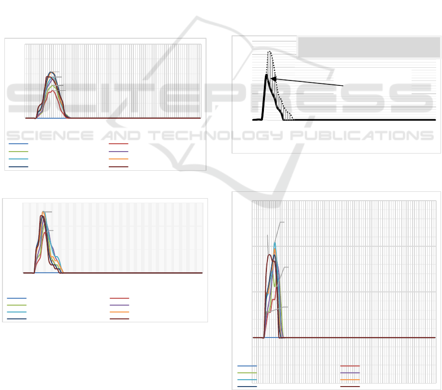
We present, in Figure 3, the delays observed in
each station for all trips of the entire journey on the
"2-Division" line after TriMet regulation. While
Figure 4 presents the delays obtained without any
regulation. It shows the contribution of the current
TriMet control. In fact, the delays are considerably
reduced (the highest value has become 15 minutes
instead of 45 minutes) and the regulation has become
faster.
Figure 3: Observed delays using TriMet regulation.
Figure 4: Observed delays with no controls.
Now we integrate our control system into the
simulator and discuss the results. After simulation,
the system detects a perturbation in the morning at
8:40 am on the 7th trip at the stop n° 1375 (SE
Division & 12th). The performance variation "F"
becomes 0.1701 which is higher than the critical
value 0.15 (This value is supposed to be fixed by the
traffic experts). We note that our system detects the
disturbance three trips earlier than TriMet (7th trip
instead of 10th trip).
After optimization, the regulator chooses "the
deviation maneuver" for all vehicles in the disturbed
area whose lowest value "F" is equal to 0.105. the list
of the regulation actions is already defined and
classified by experts (Van Oort, 2011). We note that
the same value of F was estimated by the simulator to
be 0.068 before the perturbation. We remark that the
traffic performance variation is improved by a
considerable decrease of the "F" value.
In Figure 5, we show the evolution of the observed
performance variation "F" for each trip of the traffic
with our control. The results obtained show an
improvement in the quality of service by minimizing
the values of the "F" variation during the perturbation.
The area between the two curves represents the gain
in performance variation when using our model.
Figure 5: Performance variation with TriMet and with our
control system for the 2-Division line.
Figure 6: Observed delays using our control system.
0:27
0:32
0:40
0:45
0:00
1:12
Trip 1
Trip 6
Trip 11
Trip 16
Trip 21
Trip 26
Trip 31
Trip 36
Trip 41
Trip 46
Trip 51
Trip 56
Trip 61
Trip 66
Trip 71
Trip 76
Trip 81
Trip 86
NW 5th & Davis SW 5th & Salmon
SE Division & 12th SE Division & Cesar Chavez Blvd
SE Division & 82nd SE Division & 122nd
SE Division & 162nd Gresham Transit Center
0:15
0:10
0:00
Trip 1
Trip 5
Trip 9
Trip 13
Trip 17
Trip 21
Trip 25
Trip 29
Trip 33
Trip 37
Trip 41
Trip 45
Trip 49
Trip 53
Trip 57
Trip 61
Trip 65
Trip 69
Trip 73
Trip 77
Trip 81
Trip 85
NW 5th & Davis SW 5th & Salmon
SE Division & 12th SE Division & Cesar Chavez Blvd
SE Division & 82nd SE Division & 122nd
SE Division & 162nd Gresham Transit Center
0,00
0,05
0,10
0,15
0,20
0,25
0,30
Trip 1
Trip 5
Trip 9
Trip 13
Trip 17
Trip 21
Trip 25
Trip 29
Trip 33
Trip 37
Trip 41
Trip 45
Trip 49
Trip 53
Trip 57
Trip 61
Trip 65
Trip 69
Trip 73
Trip 77
Trip 81
Trip 85
0:04
0:15
0:13
0:08
0:00
0:07
0:14
0:21
Trip 1
Trip 5
Trip 9
Trip 13
Trip 17
Trip 21
Trip 25
Trip 29
Trip 33
Trip 37
Trip 41
Trip 45
Trip 49
Trip 53
Trip 57
Trip 61
Trip 65
Trip 69
Trip 73
Trip 77
Trip 81
Trip 85
NW 5th & Davis SW 5th & Salmon
SE Division & 12th SE Division & Cesar Chavez Blvd
SE Division & 82nd SE Division & 122nd
SE Division & 162nd Gresham Transit Center
Gain in performance
variation
…….. F with current regulation
_____ F with
our
control system regulation
Agent-based Intelligent KPIs Optimization of Public Transit Control System
229
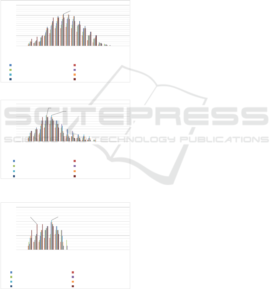
Figure 6 shows the contribution of our control
system by the considerable decrease of the delays of
the disrupted buses. It indicates that the resolution
period becomes faster. In fact, with our control
system the perturbation is completely solved at the
15
th
trip instead of the 20
th
trip.
In the following, we present in the figures below
(Fig. 7-8-9) the percentage increase of waiting
passengers per station (PI) on the disrupted trips
compared to the normal traffic without perturbation.
Figure 7: PI per station on disturbed trips with no control.
Figure 8: PI per station on disturbed trips with TriMed
control.
Figure 9: PI per station on disturbed trips with our control
system.
We note that this percentage is relatively proportional
to the bus delays. The simulation with our control
system shows a clear improvement of the service
quality by minimizing the PI value on the stations of
the disrupted trips. In fact, the number of passengers
waiting on each disrupted trip is significantly reduced
with our control system.
7 CONCLUSION AND
PERSPECTIVES
The main objective of this study was to model and
develop a transit control system. This system
simulates and controls the operational environment of
a transit network. It detects in real time the traffic
disturbances of the itineraries and generates the most
appropriate regulation action. The modelling of the
system based on a multi-agent approach dealing with
an optimization problem. The optimization resolution
includes mathematical model that describes the traffic
dynamics, and a set of constraints represents the
current traffic state. The main contribution of our
system is the multi-agent modelling of control system
using a mathematical model that treats all key
performance indicators (KPIs) as variable elements
with different weightings. To identify the variable
elements, a detailed study is conducted on the
literature of transit traffic performance measures.
To validate our control system, a simulation
model reflecting real transit dynamics was built. The
development is done with AnyLogic which is an
agent-based modelling simulator. Our model gives
visual and mathematical results justifying the choice
of the control action. The results show that the
proposed model is able to (i) evaluate the impact of
the disturbance on the transit performance and (ii)
regulate the disturbance with a better performance
than the real one.
Finally, in a perspective, we mention two tracks:
(i) to be able to manage disturbances in unfamiliar
situations (unknown disturbance, new traffic
parameter, etc.), we need to improve the behaviour of
the system by providing an evolutionary approach in
its resolution. This approach consists of making sure
that, thanks to the regulator agent, the system can
remember the results for these types of situations. The
model should then suggest a fast neighborhood
solution as a future action with new experiences and
update the regulator's knowledge base by inserting
these new rules to cope with future situations. (ii) to
orient the control system towards the operator, we
need to change the goal and include other
3,13%
0,00%
1,00%
2,00%
3,00%
4,00%
Trip 5
Trip 6
Trip 7
Trip 8
Trip 9
Trip 10
Trip 11
Trip 12
Trip 13
Trip 14
Trip 15
Trip 16
Trip 17
Trip 18
Trip 19
Trip 20
Trip 21
Trip 22
Trip 23
Trip 24
Trip 25
NW 5th & Davis SW 5th & Salmon
SE Division & 12th SE Division & Cesar Chavez Blvd
SE Division & 82nd SE Division & 122nd
SE Division & 162nd Gresham Transit Center
1,04%
1,04%
0,00%
0,50%
1,00%
1,50%
Trip 5
Trip 6
Trip 7
Trip 8
Trip 9
Trip 10
Trip 11
Trip 12
Trip 13
Trip 14
Trip 15
Trip 16
Trip 17
Trip 18
Trip 19
Trip 20
Trip 21
Trip 22
Trip 23
Trip 24
Trip 25
NW 5th & Davis SW 5th & Salmon
SE Division & 12th SE Division & Cesar Chavez Blvd
SE Division & 82nd SE Division & 122nd
SE Division & 162nd Gresham Transit Center
1,04%
0,90%
0,00%
0,50%
1,00%
1,50%
Trip 5
Trip 6
Trip 7
Trip 8
Trip 9
Trip 10
Trip 11
Trip 12
Trip 13
Trip 14
Trip 15
Trip 16
Trip 17
Trip 18
Trip 19
Trip 20
Trip 21
Trip 22
Trip 23
Trip 24
Trip 25
NW 5th & Davis SW 5th & Salmon
SE Division & 12th SE Division & Cesar Chavez Blvd
SE Division & 82nd SE Division & 122nd
SE Division & 162nd Gresham Transit Center
ICINCO 2021 - 18th International Conference on Informatics in Control, Automation and Robotics
230

performance measures related to the costs of
transport. This track consists of adapting the
optimization method to resolve a problem with
antagonistic variables. Variables directed towards the
user's view and variables directed towards the
operator's view.
REFERENCES
Mark Tromp et al, (2011) Mark Tromp, Xiang Liu and
Daniel J. Graham, “Development of Key Performance
Indicator to Compare Regularity of Service Between
Urban Bus Operators”, Transportation Research
Record Journal of the Transportation Research Board
2216(-1).
M. Napiah et al., (2015) M. Napiah,, I. Kamaruddin and
Suwardo, “Punctuality index and expected average
waiting time of stage buses in mixed traffic”, WIT
Transactions on The Built Environment, Vol 116, ©
2011 WIT Press. ISSN 1743-3509 (on-line).
Oded Cats et al., (2010) Oded Cats, Wilco Burghout, Tomer
Toledo, and Haris N. Koutsopoulos, “Mesoscopic
Modeling of Bus Public Transportation”, No. 2188,
Transportation Research Board of the National
Academies, Washington, D.C., 2010, pp. 9–18.
Neila Bhouri et al., (2016) Neila Bhouri, Maurice Aron and
Gérard Scemama, “Gini Index for Evaluating Bus
Reliability Performances for Operators and Riders”,
Transportation Research Board, Washington, 13p.
S. Carosi a, et al., (2015) S. Carosi a,, S. Gualandi b, F.
Malucelli c and E. Tresoldi, “Delay management in
public transportation: service regularity issues and crew
re-scheduling”, 18th Euro Working Group on
Transportation, EWGT, Delft, The Netherlands.
Noorfakhriah Y. and Madzlan N., (2011) Noorfakhriah
Yaakub and Madzlan Napiah, “Public Transport:
Punctuality Index for Bus Operation”, World Academy
of Science, Engineering and Technology, International
Journal of Civil and Environmental Engineering,
Vol:5, No:12.
Xumei Chen et al., (2009) Xumei Chen, Lei Yu, Yushi
Zhang, and Jifu Guo, “Analyzing Urban Bus Service
Reliability At The Stop, Route, and Network Levels”,
Transportation Research Part A 43, pp. 722–734.
Vaniyapurackal, (2015) Vaniyapurackal Jilu Joseph,
“Punctuality Index for the City Bus Service”,
International Journal of Engineering Research Volume
No.4, Issue No.4, pp: 206-208, ISSN:2319-6890.
Saberi, Meead, et al., (2013) Meead Saberi and Ali Zockaie
K., 2013. “Definition and Properties of Alternative Bus
Service Reliability Measures at the Stop Level”.
Journal of Public Transportation, 16 (1): 97-122.
Ceder, (2007) Ceder, A., “Public Transit Planning and
Operation: Theory, modelling and practice”: Elsevier
Ltd.
Zhenliang, (2013) Zhenliang Ma, Luis Ferreira and
Mahmoud Mesbah, “A Framework for the
Development of Bus Service Reliability Measures”,
Australasian Transport Research Forum, Brisbane,
Australia.
Kenneth et al., (2004) Kenneth J Dueker, Thomas J Kimpel,
James G Strathman, “Determinants of Bus Dwell
Time”, Journal of Public Transportation.
Levinson, Herbert, (1983) Levinson, Herbert. Analyzing
transit travel time performance, Transportation
Research Record 915.
Vu The Tran et al., (2012) Vu The Tran, Peter Eklund, Chris
Cook. “Toward real-time decision making for bus
service reliability”, International Symposium on
Communications and Information Technologies.
Cats et al., (2011) Cats, Nabavi, Koutsopoulos and
Burghout, “Impacts of holding control strategies on
transit performance: A bus simulation model analysis”,
Transportation Research Record Journal of the
Transportation Research Board, Pages 51-58.
Rossetti et al, (2002) Rosaldo J.F Rossetti, Rafael H.
Bordinia, Ana L. C Bazzan, Sergio Bampi, Ronghui Liu
Dirck Van Vliet. Using BDI agents to improve driver
modelling in a commuter scenario, Transportation
Research Part C: Emerging Technologies, Volume 10,
Issues 5–6, Pages 373-398.
Van Oort, (2009) N. and R. van Nes, 2009, “Control of
public transport operations to improve reliability:
theory and practice”, Transportation Research Record,
No. 2112
Ashby, W.R., (1956) Ashby, W.R., An introduction to
cybernetics, Chapman and Hall, London.
Cambridge Systematics Inc. (2005), Cambridge
Systematics Inc., PB Consult Inc., and System Metrics
Group. Analytical tools for asset management. 545,
NCHRP report, 2005.
European Commission, (2011) European Commission.
White paper - Roadmap to a single European Transport
Area - Towards a competitive and resource efficient
transport system.
Yan et al., (2009) Yan, XY and Crookes, RJ. Reduction
potentials of energy demand and GHG emissions in
China's road transport sector. Energy Policy, Vol. 37,
2009, pp. 658-668.
Noorfakhriah Y. and Madzlan N., (2011) Noorfakhriah
Yaakub and Madzlan Napiah, “Public Transport:
Punctuality Index for Bus Operation”, World Academy
of Science, Engineering and Technology, International
Journal of Civil and Environmental Engineering, Vol:5.
Saberi, Meead, et al, (2013) Meead Saberi and Ali Zockaie
K., 2013. “Definition and Properties of Alternative Bus
Service Reliability Measures at the Stop Level”.
Journal of Public Transportation, 16 (1): 97-122.
Van Oort (2011), Service reliability and urban public
transport, this research is supported by HTM (the public
transport company in The Hague), Delft University of
Technology (department of Transport & Planning),
TRAIL (research school for transport, infrastructure
and logistics), Goudappel Coffeng (mobility
consultants), the Transport Research Centre Delft and
Railforum.
Agent-based Intelligent KPIs Optimization of Public Transit Control System
231
