Viscoelastic Fluid Simulation based on the Combination of Viscous and

Elastic Stresses

Nobuhiko Mukai

1,2,3

, Ren Morooka

, Takuya Natsume

and Youngha Chang

1,2

Computer Science, Tokyo City University, 1-28-1 Tamazutsumi, Setagaya, Tokyo, Japan

Graduate School of Integrative Science and Engineering, Tokyo City University,

1-28-1 Tamazutsumi, Setagaya, Tokyo, Japan

Institute of Industrial Science, the University of Tokyo, 4-6-1, Komaba, Meguro, Tokyo, Japan

Keywords:

Particle Method, Viscoelastic Fluid, Spinnability, Cauchy’s Equation of Motion, Constitutive Equation.

Abstract:

It is one of the challenging issues to simulate and visualize liquid behavior, especially the behavior of the

viscoelastic ﬂuid because it has both characteristics of viscosity and elasticity. Although Newtonian ﬂuid,

which sharing stress is proportional to the velocity gradient, is often analyzed with the ordinal governing

equations that are Navier-Stokes equation and the equation of continuity, viscoelastic ﬂuid behavior is so

complex that there are no established governing equations, especially for the constitutive equation. Then,

some studies used the Finite Element Method, and others developed a point-based method. In addition, the

viscoelastic ﬂuid has a unique characteristic called “Spinnability”. The ﬂuid is stretched so long like a string

and shrinks very fast when it is ruptured. Therefore, we have been performing viscoelastic ﬂuid simulations

based on Cauchy’s equation of motion by devising the stress term in the constitutive equation. In this paper,

we report a viscoelastic ﬂuid simulation based on the combination of viscous and elastic stresses.

1 INTRODUCTION

Computer graphics can visualize almost all of the

things from artiﬁcial objects to natural phenomena.

However, the visualization has no meaning without

precise simulations. One of the most difﬁcult and

challenging issues is to simulate and visualize liquid

behavior precisely, because the liquid shape changes

dynamically and its boundary is very clear. In the

liquid simulations, Newtonian ﬂuid is comparatively

simple since the relation between the shearing stress

and the velocity gradient is linear.

However, there are many non-Newtonian ﬂuids

in the world, and one of them is called “viscoelas-

tic ﬂuid” that has two characteristics of viscosity and

elasticity, and the relation between the shearing stress

and the velocity gradient is not linear. The behav-

ior is so complex that there are no established gov-

erning equations, especially for the constitutive equa-

tion. There are some studies that use FEM (Finite

Element Method) or SM (Spring Mass) model, and

others employ several kinds of methods such as a

point-based method. In addition, the viscoelastic ﬂuid

has a unique characteristic called “spinnability”. The

ﬂuid can be stretched so long as if it is a string, and

then it shrinks very fast when it is ruptured. There is

no previous work that can represent the behavior of

spinnability.

Then, we have been trying to simulate and visu-

alize the behavior of spinnability based on Cauchy’s

equation of motion. In the equation, there is a term

of “deviatoric stress”, which should be composed of

viscous and elastic stresses, because the viscoelastic

ﬂuid has two characteristics of viscosity and elastic-

ity. In our previous works, we treated the deviatoric

stress as a linear combination of viscous and elastic

stresses, where the sum of the coefﬁcients for viscos-

ity and elasticity equals to 1.0.

On the other hand, the behavior of the viscoelastic

ﬂuid suddenly changes at the rupture point when

it begins to be ruptured. Therefore, in this paper,

we decide the coefﬁcients of the linear combination

of viscous and elastic stresses experimentally, and

show the comparison of the simulation results for

several kinds of parameters with real viscoelastic

ﬂuid behavior.

172

Mukai, N., Morooka, R., Natsume, T. and Chang, Y.

Viscoelastic Fluid Simulation based on the Combination of Viscous and Elastic Stresses.

DOI: 10.5220/0010615901720178

In Proceedings of the 11th International Conference on Simulation and Modeling Methodologies, Technologies and Applications (SIMULTECH 2021), pages 172-178

ISBN: 978-989-758-528-9

2 RELATED WORKS

Related to Newtonian ﬂuid works, there is a survey

that shows two types of studies: hydrodynamic theory

based research and experimental based works (Mould

and Yang, 1997), and also there is another investi-

gation published during the 1980s and 1990s (Igle-

sias, 2004). In addition, there is a survey on com-

puter graphics based ocean simulations and the ren-

dering (Darles et al., 2011), which shows two types

of methods: physics based methods using Navier-

Stokes equation and empirical law based oceano-

graphic methods.

Some people employed a mesh modeling to rep-

resent ocean waves (Hinsinger et al., 2002), irregular

long crest waves (Cui et al., 2004), and vast ocean

scene (Dupuy and Bruneton, 2012), because ocean

waves have continuous smooth surfaces. The draw-

back of the mesh modeling is re-meshing that takes

a lot of time and is necessary when the topology

changes. Then, others utilized a particle method. SPH

(Smoothed Particle Hydrodynamics) is one of the par-

ticle methods, and they presented water pouring into

a glass (M

uller et al., 2003) and river ﬂowing (Kipfer

and Westermann, 2006).

As for the ﬂuid behavior simulations, there are

two kinds of methods: Eulerian (grid based) and La-

grangian (particle based) methods. There are some

studies that utilized Eulerian method to propose an

optimized grid for GPU (Graphics Processing Unit)

(Chentanez and M

uller, 2010a) and to represent freez-

ing ice with air bubbles (Nishino et al., 2012). On

the other hand, there are other studies that employed

semi-Lagrangian method to represent viscous liq-

uids interacting with 3D objects (Foster and Fedkiw,

2001) and to represent bubbles with Voronoi diagram

(Busaryev et al., 2012).

Moreover, other people used a hybrid method of

Eulerian and Lagrangian to represent bubbles in wa-

ter (Hong et al., 2008) and spray or splash (Chentanez

and M

uller, 2010b). There is also a method to animate

viscous ﬂuid with collision between particles and ob-

stacles (Miller, 1989), and a parallel particle render-

ing system that allows to treat particles with different

shapes, sizes, colors and transparencies (Sims, 1990).

In addition, some studies proposed particle level-set

algorithms to visualize many kinds of bubble shapes

(Greenwood and House, 2004) and ﬁne splash parti-

cles (Geiger et al., 2006). There are also some works

that employed a level set method to present bubbles in

liquid and gas interaction (Kim et al., 2007), and that

also used a particle level set method for dense liquid

volume and utilized a particle method for the diffused

regions (Losasso et al., 2008).

For the simulations of the viscoelastic ﬂuid, some

people used a spring-mass system to visualize an egg

dropping on the ﬂoor (Tamura et al., 2005), and others

employed Finite Element methods to represent large

plastic deformation of solid materials and to simulate

the complex elastic and plastic behavior of viscoelas-

tic materials (Bargtei et al., 2007) (Wojtan and Turk,

2008). These utilized Eulerian method.

On the other hand, there is a study that employed

a particle based method for a viscoelastic ﬂuid sim-

ulation (Clavet et al., 2005); however, the method

also added springs to accomplish elastic and non-

linear plastic effects. The other research proposed a

new method called “Material Point Method” to sim-

ulate foams and sponges, and employed Oldroyd-B

model to preserve the plastic volume (Ram et al.,

2015). There is also another method that developed a

constrained dynamics solver by extending a position

based dynamics method to represent whipped cream

and strawberry syrup (Barreiro et al., 2017). These

methods are particle methods or hybrid methods, and

these studies do not obey Navier-Stokes equation as

the governing equation, although some works employ

the conservation of mass and momentum.

In addition, there is a research that used a grid

based method with level set to animate viscoelastic

ﬂuids such as mucus, liquid soap, and so on (Goktekin

et al., 2004). On the other hand, there is another work

that utilized SPH based method to visualize melting

and ﬂowing of the viscoelastic ﬂuid (Chang et al.,

2009). Although these studies used different meth-

ods, they both employed Navier-Stokes equation as

the governing equation, because the viscoleastic ﬂuid

has the characteristics of liquid and Navier-Stokes

equation is the established governing equation to an-

alyze ﬂuid behavior. In addition, they added viscosity

and elasticity terms to Navier-Stokes equation as the

external term.

Navier-stokes equation is the established govern-

ing equation of ﬂuid, and the viscoelastic ﬂuid has

two characteristics of viscosity and elasticity. Viscos-

ity is a feature of ﬂuid, while elasticity is another fea-

ture of elastic body that is a kind of continuum. Then,

the governing equation of the viscoelastic ﬂuid should

be Cauchy’s equation of motion, which is the funda-

mental equation of Navier-Stokes equation including

“deviatoric stress” that has both viscous and elastic

stresses.

Therefore, we have been trying to simulate the be-

havior of the viscoelastic ﬂuid by introducing a linear

combination of viscosity and elasticity for deviatoric

stress term of Cauchy’s equation of motion, and to

evaluate the stretched length of the viscoelastic ﬂuid

to visualize spinnability (Mukai et al., 2010) (Mukai

Viscoelastic Fluid Simulation based on the Combination of Viscous and Elastic Stresses

173

et al., 2018) (Mukai et al., 2019). In the previous

work, the sum of the coefﬁcients of the linear com-

bination of viscosity and elasticity was 1.0, since the

deviatoric stress is composed of viscous and elastic

stresses.

However, the behavior of the viscoelastic ﬂuid

changes dynamically between before and after the

rupture. When the ﬂuid is ruptured after being

stretched, it shrinks very fast. In the behavior of the

viscoelastic ﬂuid, the effect of viscosity is larger than

that of elasticity all the time; however the effect of

elasticity becomes a little bit larger after it is ruptured

because the ﬂuid shrinks very fast and the character-

istics of elasticity appear. Then, in this simulation,

the coefﬁcients of the linear combination of viscos-

ity and elasticity are decided experimentally, and we

show the simulation results with the different coefﬁ-

cients and the comparison of them with real viscoelas-

tic ﬂuid behavior.

3 METHOD

We employ MPS (Moving Particle Semi-implicit)

method for the simulation, which is one of parti-

cle methods and was developed by Koshizuka and

Oka for incompressible ﬂuid analysis (Koshizuka and

Oka, 1996). In this research, the governing equations

are the equation of continuity (Eq.(1)) and Cauchy’s

equation of motion (Eq.(2)), which are described in

the following.

Equation of continuity:

dρ

= 0 (1)

Cauchy’s equation of motion with surface tension:

= ∇ · σ

σ + g

g + f

f = (−∇pI

I + ∇· τ

τ) + g

g + f

f (2)

where, ρ is the density, t is time, v

v is the velocity, σ

is the stress tensor, g

g is the gravity, f

f is the external

force, p is the pressure, I

I is the unit matrix, and τ

τ is

the deviatoric stress.

The target is the viscoelastic ﬂuid that has two

characteristics of viscosity and elasticity. Then,

τ should have two characteristics of viscosity and

elasticity and can be written as follows (Eqs.(3)-(8)).

τ = ατ

+ βτ

(3)

= 2η

D (4)

D =

L + L

), L

L = ∇V

V (5)

V = (u

u,v

v,w

w) (6)

∇V

V =







∂u

∂x

∂u

∂y

∂u

∂z

∂v

∂x

∂v

∂y

∂v

∂z

∂w

∂x

∂w

∂y

∂w

∂z







(7)

= 2µε

ε, µ =

2(1 + ν)

(8)

where, τ

and τ

are viscous and elastic terms of de-

viatoric stress, respectively, and α and β are the linear

combination coefﬁcients. η

is zero shear viscosity,

V is the particle velocity, ε

ε is the distortion tensor, E

is Young’s modulus and ν is Poisson’s ratio.

In our previous study (Mukai et al., 2019),

α + β = 1 because viscoelastic stress is composed of

viscous and elastic stresses. However, the behavior

of viscosity and elasticity is different, and the effect

of viscosity is dominant all the time, while the ef-

fect of elasticity becomes a little bit larger after the

ﬂuid is ruptured since it shrinks very fast like a rub-

ber, which shows the characteristics of elasticity and

is called “spinnability”. Then, in this research, we de-

cide the parameters of α and β experimentally. The

value of α is larger than that of β all the time, because

the effect of viscosity is dominant. On the other hand,

the value of β depends on the density of the narrowest

part of the ﬂuid, because the ﬂuid shrinks very fast at

the middle part of it. Then, β can be calculated with

the following equation (Eq.(9)).

β =



1 −



C (9)

where, n

is the initial particle number density, n

the particle number density of the narrowest part at

the time k, and C is the dominant coefﬁcient for elas-

ticity, which is decided experimentally.

4 HIGH PRECISION

CALCULATION

The original MPS method developed by Koshizuka

and Oka (Koshizuka and Oka, 1996) assumes that the

particles are regularly arranged. Then, the calculation

becomes unstable when the particle arrangement is

imbalanced. In this study, we adopt some high order

MPS methods to stabilize the calculation even when

the particle arrangement is imbalanced. One of the

stabilization is for the Poisson equation of pressure

SIMULTECH 2021 - 11th International Conference on Simulation and Modeling Methodologies, Technologies and Applications

174

calculation. We use the model with the velocity di-

vergence term, which was proposed by Tanaka and

Masunag (Tanaka and Masunaga, 2010).

The original Laplacian of pressure developed by

Kishizuka and Oka (Koshizuka and Oka, 1996) was

as folllows (Eq.(10)).

< ∇

P >

k+1

∆t

− n

(10)

where, < ∇

P >

k+1

is the Laplacian of the pressure

for a particle i at the time step k + 1, ∆t is the time

step, n

is the particle number density of a particle i

at the time step k. On the other hand, the Laplacian

of pressure is calculated as follows (Eq.(11)) by the

method proposed by Tanaka and Masunaga (Tanaka

and Masunaga, 2010).

< ∇

P >

k+1

∆t

∇ · u

∗

+ γ

∆t

− n

(11)

where, u

∗

is the provisional velocity vector of the par-

ticle i, and γ is the relaxation coefﬁcient, which is set

depending on the problem. In this simulation, it is

set as 0.2 according to the pre-calculation result. For

an ideal incompressible ﬂuid, ∇ · u

u equals to 0; how-

ever, in computer simulations, it does not equal to 0.

Then, Eq.(11) considers the term for the precise pres-

sure calculation.

The other stabilization is for the calculation of the

pressure gradient. For this purpose, we employ a high

order gradient model developed by Iribe and Nakaza

(Iribe and Nakaza, 2011). Moreover, in order to pre-

vent the excessive approach of particles, the model

developed by Monaghan (Monaghan, 2000) is used,

which considers the artiﬁcial repulsive force that is

added to the gradient model developed by Iribe and

Nakaza (Iribe and Nakaza, 2011). The original gradi-

ent of the pressure developed by Koshizuka and Oka

(Koshizuka and Oka, 1996) was as follows (Eq.(12)).

< ∇P >

∑

j6=i

−

− r

)ω(|r

− r

|) (12)

On the other hand, the high order pressure gradi-

ent is calculated with the method developed by Mon-

aghan (Monaghan, 2000) in the following (Eq.(13)).

< ∇P >

∑

j6=i

− r

)

− r

⊗

− r

)

− r

ω(|r

− r

−1

∑

j6=i

−

− r

)ω(|r

− r

(13)

where, ⊗ is the tensor product, and

is the mini-

mum pressure in the radius of inﬂuence so that

always lower than P

. Since P

−

is always posi-

tive, the repulsive force is generated between particles

i and j Then, it is possible to prevent the excessive ap-

proach of particles due to the attraction. Eq.(13) en-

ables the calculation stable by replacing d in Eq.(12)

with the inverse matrix in Eq.(13). By the calculation

with Eq.(13), the pressure becomes stable even when

particles are not regularly arranged, and the inverse

matrix becomes a unit matrix when particles are reg-

ularly arranged. In this case, Eq.(13) is equivalent to

Eq.(12).

5 SIMULATION

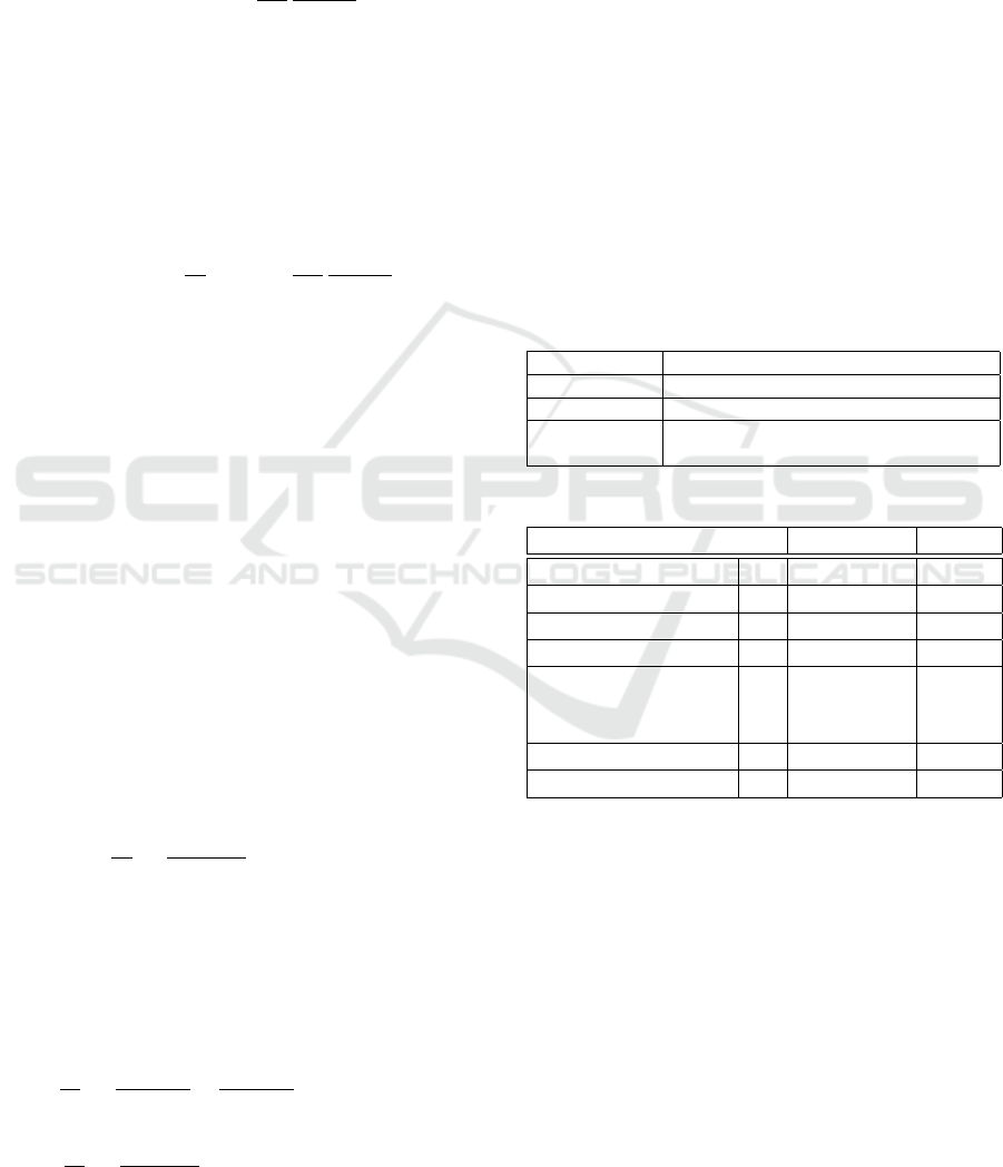
Table 1 and 2 show the speciﬁcations of the PC and

the parameters used for the simulation, respectively.

Table 1: Speciﬁcation of the PC used in the simulation.

OS Windows 10 Education 64 bit

CPU Intel Core i5-8400 2.8GHz

Main memory 8GB

GPU GeForce GTX 1660 SUPER with 6GB

memory

Table 2: Parameters used for the simulation.

Parameter Value Unit

Density ρ 1.16 × 10

−3

g/mm

Young’s modulus E 1.05 × 10

Poisson’s ratio ν 0.5

Zero shear viscosity η

28 Pa · s

Initial distance

of particles

(= Particle radius)

0.3 mm

Pulling velocity v

v 18 mm/s

Time step 4t 0.10 × 10

−3

Fig.1 shows the initial state of the particles, and

(a) shows the side view for all particles. In the side

view, the upper squared part of the particles is a solid

body that is pulled up with the pulling velocity. On

the other hand, the lower larger squared part of the

particles is a rigid body that does not move even if

other part of the particles moves. The middle cubed

part of the particles is the viscoelastic ﬂuid that is

pulled according to the upper squared part of the

particles. On the other hand, Fig.1 (b) shows the

top view for only the viscoelastic ﬂuid, which has

four side named S1, S2, S3 and S4, which side has

three particle width. In this research, we assume

that the viscoelastic ﬂuid begins to be ruptured if the

particles enter in the radius of inﬂuence of the particle

Viscoelastic Fluid Simulation based on the Combination of Viscous and Elastic Stresses

175

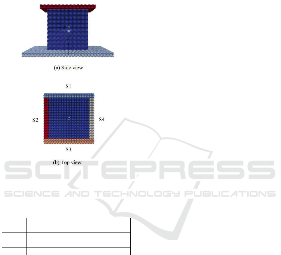
in the confrontation. For example, if the particle

in S1 enters in the radius of inﬂuence of the par-

ticle in S3, the viscoelastic ﬂuid begins to be ruptured.

Figure 1: Initial state of particles.

Table 3 shows the speciﬁcation of the particles

shown in Fig.1.

Table 3: Particle speciﬁcation.

Part Size [mm]

(Width×Depth×Hight)

# of particles

Upper 12.3×12.3×0.9 5,043

Middle 9.3× 9.3×9.3 29,791

Lower 18.9×18.9×0.9 11,907

6 RESULTS

In the simulation, we used 0.97 and 0.95 as α for be-

fore and after the rupture of the stretched viscoelastic

ﬂuid, respectively. The value of α is large because we

have found experimentally that the effect of viscosity

is larger than that of elasticity all the time. In addition,

if α is larger than 0.97, viscoelastic ﬂuid behaves as if

it is Newtonian ﬂuid, and it ﬂows down on the ﬂoor.

It does not show the characteristic of elasticity if α is

larger than 0.97. In addition, the effect of elasticity

becomes a little bit larger after the rupture, because

the characteristics of elasticity appear and the ﬂuid

shrinks very fast like a rubber. This means that the

characteristics of viscosity become a little bit lower

compared with that in the before. Then, the value of

α after the rupture is lower than that before the rup-

ture.

On the other hand, β is decided with Eq.(9), and

the maximum value is C when the particle number

density n

is 0, which means that stretched viscoelas-

tic ﬂuid is completely ruptured. Then, we set 0.03,

0.05 and 0.07 as C. One reason is that 0.03+0.97=1,

which means that 0.03 is the complement of 0.97 that

is the value of α before the rupture. The second rea-

son is that 0.05+0.95=1, which means that 0.05 is the

complement of 0.95 that is the value of α after the rup-

ture. Setting 0.07 as C is the conﬁrmation that the ef-

fect of viscosity is too strong for the viscoelastic ﬂuid

to be stretched, because 0.07+0.95=1.02>1.0.

Fig.2 shows the three kinds of simulation images

after 750 steps and a real viscoelastic ﬂuid named

“guar gum”.

In Fig.2 (a), (b), and (c), the middle part width be-

comes thinner as C becomes larger, because larger C

means the less effectiveness of viscosity and the more

effectiveness of elasticity. All the stretched lengths of

three images are shorter than a real viscoelastic ﬂuid

shown in Fig.2 (d). Spinnability, which is a unique

characteristic of viscoelastic ﬂuid, has three features:

1) it can be stretched very long, 2) the middle part

of it becomes very thin, and 3) it shrinks very fast

when it is ruptured. In the simulation results, it seems

that the feature 2) is satisﬁed; however, the feature

1) is not satisﬁed. All three stretched lengths are

shorter than the real viscoelastic ﬂuid shown in (d).

In fact, the stretched length in the simulation using

C = 0.05 was 1.4[mm], while the real viscoelastic

ﬂuid stretched length was 41.8[mm] that was mea-

sured in the movie. In the feature 3), the shrinking

time in the simulation using C = 0.05 was 500[ms],

while it was 4, 333[ms] in the real viscoelastic ﬂuid,

which means that the viscoelastic ﬂuid in the simu-

lation shrunk faster than the real ﬂuid, although it is

partly due to the shorter stretching than that of the real

ﬂuid. As a result, the effect of viscosity should be

stronger than that of elasticity to realize spinnability

in the viscoelastic ﬂuid simulation. However, the too

large value of α makes the viscoelastic ﬂuid behave

as if it is Newtonian ﬂuid.

7 CONCLUSIONS

In this paper, we have adopted two high order cal-

culations of pressure to simulate the behavior of the

viscoelastic ﬂuid precisely. One is for Laplacian of

SIMULTECH 2021 - 11th International Conference on Simulation and Modeling Methodologies, Technologies and Applications

176

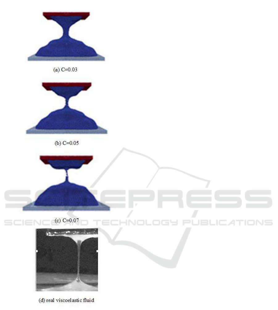
Figure 2: Simulation results and a real viscoelastic ﬂuid.

pressure that is used in the Poisson equation, and the

other is for the gradient of pressure, which prevents

the excessive approach of particles. In the simula-

tion of the viscoelastic ﬂuid behavior, we have em-

ployed the idea of the combination for viscous and

elastic stresses of deviatoric stress; however, the coef-

ﬁcients of the combination were decided experimen-

tally keeping the sum of coefﬁcients equals to almost

1.0.

As the result of the simulation, one of the features

in spinnability was satisﬁed, and the middle part of

the ﬂuid became very thin. However, the stretched

length in the simulation was shorter than that in the

real ﬂuid, and the shrinking time in the simulation

was also shorter. One of the reasons is the shortage

of the particles used in the simulation to realize the

precise behavior of viscoelastic ﬂuid. Although the

simulation results differed from the behavior of the

reawhich arel viscoelastic ﬂuid “guar gum”, we have

conﬁrmed that the combination of viscous and elastic

stresses can be one solution for the analysis of vis-

coelastic stress. In this paper, the linear combination

coefﬁcients of α and β, and the elastic dominant co-

efﬁcient of C were decided experimentally; however,

these coefﬁcients shoud be decided theoretically with

some evidence.

In the future, we have to reconsider the combina-

tion way of viscous and elastic stresses in deviatoric

stress term to realize the two remaining characteristics

of spinnability, and we also have to use more particles

to simulate viscoelastic ﬂuid behavior precisely.

REFERENCES

Bargtei, A., Wojtan, C., Hodgins, J., and Turk, G. (2007). A

ﬁnite element method for animating large viscoplastic

ﬂow. ACM Transactions on Graphics, 26(3):Article

No.16.

Barreiro, H., Garc

ıa-Ferm

andez, I., Aldu

an, I., and Otaduy,

M. (2017). Conformation constraints for efﬁcient

viscoelastic ﬂuid simulation. ACM Transactions on

Graphics, 36(6):Article No.221.

Busaryev, O., Dy, T., Wang, H., and Ren, Z. (2012). An-

imating bubble interactions in a liquid foam. ACM

Transactions on Graphics, 31(4):63:1–63:8.

Chang, Y., Bao, K., Liu, Y., Zhu, J., and Wu, E. (2009).

A particle-based method for viscoelastic ﬂuids anima-

tion. In ACM Symposiumon virtual reality software

and technology, pages 463–468.

Chentanez, N. and M

uller, M. (2010a). Real-time simu-

lation of large bodies of water with small scale de-

tails. In ACM SIGGRAPH/Eurographics symposium

on computer animation, pages 197–206.

Chentanez, N. and M

uller, M. (2010b). Real-time simula-

tion of large bodies of water with small scale details.

Clavet, S., Beaudoin, P., and Poulin, P. (2005). Particle-

based viscoelastic ﬂuid simulation. In ACM SIG-

GRAPH/Eurographics Symposium on computer ani-

mation, pages 219–228.

Cui, X., Yi-cheng, J., and Xiu-wen, L. (2004). Real-

time ocean wave in multi-channel marine simulator.

In ACM SIGGRAPH international conference on vir-

tual reality continuum and its application in industry,

pages 332–335.

Darles, E., Crespin, B., Ghazanfarpour, D., and Gonzato,

J. (2011). A survey of ocean simulation and rendering

Viscoelastic Fluid Simulation based on the Combination of Viscous and Elastic Stresses

177

techniques in computer graphics. In Computer Graph-

ics Forum, volume 30, pages 43–60.

Dupuy, J. and Bruneton, E. (2012). Real-time animation and

rendering of ocean whitecaps. In SIGGRAPH Asia,

Technical Briefs, page Article No.15.

Foster, N. and Fedkiw, R. (2001). Practical animation of

liquids. In ACM SIGGRAPH, pages 23–30.

Geiger, W., Leo, M., Rasmussen, N., Losasso, F., and Fed-

kiw, R. (2006). So real it’ll make you wet. In ACM

SIGGRAPH Sketches, page Article No.20.

Goktekin, T., Bargteil, A., and O’Brien, J. (2004). A

method for animating viscoelastic ﬂuids. ACM Trans-

actions on Graphics, 23(3):463–468.

Greenwood, S. and House, D. (2004). Better with bubbles:

Enhancing the visual realism of simulated ﬂuid. In

ACM SIGGRAPH/Eurographics symposium on com-

puter animation, pages 287–296.

Hinsinger, D., Neyret, F., and Cani, M. (2002). Inter-

active animation of ocean waves. In ACM SIG-

GRAPH/Eurographics symposium on computer ani-

mation, pages 116–166.

Hong, J., Lee, H., Yoon, J., and Kim, C. (2008). Bubbles

alive. ACM Transactions on Graphics, 27(3):48:1–

48:8.

Iglesias, A. (2004). Computer graphics for water modeling

and rendering: A survey. Future Generation Com-

puter Systems, 20(8):1355–1374.

Iribe, T. and Nakaza, E. (2011). An improvement of accu-

racy of the mps method with a new gradient calcula-

tion model (in japanese). Journal of the Japan Society

of Civil Engineers(B2), 67(1):36–48.

Kim, B., Liu, Y., Llamas, I., Jiao, X., and Rossignac, J.

(2007). Simulation of bubbles in foam with the vol-

ume control method. ACM Transactions on Graphics,

26(3):98:1–98:10.

Kipfer, P. and Westermann, R. (2006). Realistic and interac-

tive simulation of rivers. In Graphics Interface, pages

41–48.

Koshizuka, S. and Oka, Y. (1996). Moving-particle semi-

implicit method for fragmentation of incompressible

ﬂuid. Nuclear Science and Engineering, 123:421–

434.

Losasso, F., Talton, J., Kwatra, N., and Fedkiw, R. (2008).

Two-way coupled sph and particle level set ﬂuid simu-

lation. IEEE Transsactions on Visualization and Com-

puter Graphics, 14(4):797–804.

Miller, G. (1989). Globular dynamics: A connected parti-

cle system for animating viscous ﬂuids. Computers &

Graphics, 13(3):305–309.

Monaghan, J. (2000). SPH without a tensile instability.

Journal of Computational Physics, 159(2):290–311.

Mould, D. and Yang, Y. (1997). Modeling water for com-

puter graphics. Computers & Graphics, 21(6):801–

814.

uller, M., Charypsr, D., and Gross, M. (2003). Particle-

based ﬂuid simulation for interactive applications. In

ACM SIGGRAPH/Eurographics symposium on com-

puter animation, pages 154–159.

Mukai, N., Ito, K., Nakagawa, M., and Kosugi, M. (2010).

Spinnability simulation of viscoelastic ﬂuid. In ACM

SIGGRAPH Posters, page Article No.18.

Mukai, N., Matsui, E., and Chang, Y. (2019). Investigation

on viscoelastic ﬂuid behavior by modifying deviatoric

stress tensor. In SIMULTECH, pages 216–222.

Mukai, N., Nishikawa, T., and Chang, Y. (2018). Evaluation

of stretched thread lengths in spinnability. In ACM

SIGGRAPH Posters, page Article No.62.

Nishino, T., Iwasaki, K., Dobashi, Y., and Nishita, T.

(2012). Visual simulation of freezing ice with air bub-

bles. In SIGGRAPH Asia, Technical Briefs, page Ar-

ticle No.1.

Ram, D., Gast, T., Jiang, C., Schroeder, C., Sromakhin, A.,

Teran, J., and Kavehpour, P. (2015). A material point

method for viscoelastic ﬂuids, foams and sponges. In

ACM SIGGRAPH/Eurographics symposium on com-

puter animation, pages 157–163.

Sims, K. (1990). Particle animation and rendering using

data parallel computation. In ACM SIGGRAPH, vol-

ume 24, pages 405–413.

Tamura, N., Tsumura, N., Nakaguchi, T., and Miyak, Y.

(2005). Spring-bead animation of viscoelastic ma-

terials. In ACM SIGGRAPH Sketches, page Article

No.64.

Tanaka, M. and Masunaga, T. (2010). Stabilization and

smoothing of pressure in mps method by quasi-

compressibility. Journal of Computational Physics,

229(11):4279–4290.

Wojtan, C. and Turk, G. (2008). Fast viscoelastic behavior

with thin features. ACM Transactions on Graphics,

27(3):Article No.47.

SIMULTECH 2021 - 11th International Conference on Simulation and Modeling Methodologies, Technologies and Applications

178