A Longitudinal Model for Song Popularity Prediction

Ahmet Çimen

and Enis Kayış

Department of Industrial Engineering, Ozyegin University, Istanbul, Turkey

Keywords: Music Analytics, Time-varying Coefficients, Mathematical Programming.

Abstract: Usage of new generation music streaming platforms such as Spotify and Apple Music has increased rapidly

in the last years. Automatic prediction of a song’s popularity is valuable for these firms which in turn translates

into higher customer satisfaction. In this study, we develop and compare several statistical models to predict

song popularity by using acoustic and artist-related features. We compare results from two countries to

understand whether there are any cultural differences for popular songs. To compare the results, we use

weekly charts and songs’ acoustic features as data sources. In addition to acoustic features, we add acoustic

similarity, genre, local popularity, song recentness features into the dataset. We applied Flexible Least Squares

(FLS) method to estimate song streams and observe time-varying regression coefficients using a quadratic

program. FLS method predicts the number of weekly streams of a song using the acoustic features and the

additional features in the dataset while keeping weekly model differences as small as possible. Results show

that the significant changes in the regression coefficients may reflect the changes in the music tastes of the

countries.

1 INTRODUCTION

The music industry is expanding every day with new

artists, songs, and listeners. The growth of the music

industry has been increasing since 2014 with the

impact of music streaming services on preventing

piracy (Stone, 2020). In 2020, half of the revenue of

the industry is generated by these services and at the

end of 2020 over 70 million songs were available in

the leading music stream service, Spotify, with a

market coverage of 170 countries. (Spotify, 2021)

Increasing popularity of online music streaming

services allows listeners to access newly released

songs around the world besides the old ones. Hence

the increasing variety of artists, song genres, and

songs generate a vast amount of data with the help of

the digitalization of the music industry

Music streaming services expanded their

customer base with the increasing trend of paid media

services. Increasing number of users creates higher

number of streams for the songs which helps the

music economy to grow. Meanwhile some of these

services losing their share in the market, Apple

Music, Spotify, and YouTube Music are becoming

https://orcid.org/0000-0003-3395-6685

https://orcid.org/0000-0001-8282-5572

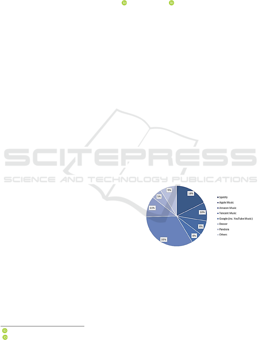
more popular than ever. At the beginning of 2020,

Spotify got 32-34% of the market which makes

Spotify the market leader with 345 million users.

(Mulligan, 2020).

Figure 1: Market share of the music streaming services in

2020.

These platforms collect and store usage

information about the users. Besides, some acoustic

numerical features are generated out of the songs by

these platforms. All this collected information allows

developers/researchers to analyze the music listening

habits, detect the hit songs/genres, and develop

musical insights for producers, listeners, and artists.

To increase user engagement and satisfaction, it is

Çimen, A. and Kayı¸s, E.

A Longitudinal Model for Song Popularity Prediction.

DOI: 10.5220/0010607700960104

In Proceedings of the 10th International Conference on Data Science, Technology and Applications (DATA 2021), pages 96-104

ISBN: 978-989-758-521-0

crucial to analyze music tastes. The music taste of the

audience differs between countries and changes over

time. Acoustic features, historical events, seasons,

holidays, and social influence are factors that may

affect a song’ popularity. Naturally, the effects of

these factors are dynamic and culture-specific. In

different countries, song popularity may be affected

by these factors differently over time. Geographical

and cultural distances between countries affect the

popularity of the songs. (Buda and Jarnowski, 2015)

In this paper, we used a time-varying penalized

regression model to predict the number of song

streams using acoustic features gathered using

Spotify API and monitor the regression parameters

over a period to discover the effects of the acoustic

features on the music taste. Our approach allows us to

smooth the extreme changes of the regression

parameters over time so that the shifts in the musical

preferences are reflected realistically. We also

compared the results for two countries; Turkey and

the U.S. to observe the cross-cultural differences in

the music tastes.

The rest of the paper is organized as follows.

Section 2 provides a review of related literature.

Section 3 describes the problem that we have worked

on and explains the methodology that we have used.

Section 4 explains the data scraping and preparation

steps and the results of the regression model. Finally,

Section 5 concludes the paper and discusses future

works.

2 RELATED WORK

Our motivation is to examine cross-cultural music

preferences and their shifts over time by using the

charts data and the acoustic features of songs.

Previous works that focused on similar problems exist

in the literature and the methodologies that they

follow in these works vary. There are applications of

predictive algorithms and survey-based approaches

for understanding the Spatio-temporal music

preferences of different populations.

A regression-based approach is used by (Suh,

2019) with Spotify’s acoustic features to predict

songs’ success on the charts. They use OLS

regression for prediction and analyse variable

significances for 6 different countries. (Pınarbaşı,

2019) analyse music popularity characteristics of

Turkey for a 6-month period by using decision tree

algorithm. They also cluster the acoustic features

gathered from the Spotify and concluded with 3

different clusters with similar acoustic features.

(Yadati et al., 2017) focuses on the change of the

musical preferences when the mood/activity change.

Their findings show that the acoustic features of the

songs and the genre/instrument information are not

sufficient for predicting the mood/activity change.

Classification models are also applied to predict

whether a song is a hit or not. A similar work from

(Al-Beitawi et al., 2020) shows that the musical

attributes from Spotify may help clustering the songs

and discovering the acoustic features that have

influence on the song popularity such as high

danceability and low instrumentalness. (Herremans

et al., 2014) compare classification methods such as

SVM, Naïve Bayes, logistic regression, and decision

tree for hit song prediction. Their dataset includes

Billboard’s Hot 100 charts with the acoustic features

from The Echo Nest which is owned by Spotify.

Same acoustic features used for analyzing the music

popularity by (Sciandra and Spera 2020). They

applied a Beta GLMM to detect the features that have

effects on song popularity. They found out that

energy, valence, and duration features affect the song

popularity positively. (Ni et al. 2011) discovered that

the hit songs having higher tempo and getting louder

over time as a result of their binary classification

study. However, their findings showed that over a 50-

years period harmonically simple songs are more

likely to be hit.

There are also works that are not data driven.

(LeBlanc et al., 2000) tested the music listening

preferences by surveying young listeners around 5

countries. They found that the tempo of the song,

listener’s age and country affect the music preference.

(Rentfrow and Gosling, 2003) collected over 3500

samples from different geographical regions and

discover 4 music preference dimensions such as

Reflective and Complex, Intense and Rebellious,

Upbeat and Conventional and Energetic and

Rhythmic. They explained and related the music

preferences with the personal characteristics, political

views, and cognitive abilities.

Time-varying coefficient models such as Kalman

filters, smoothing spline methods and time-varying

coefficient regressions are widely used to analyse

longitudinal data in different domains.

Ordinary Least Squares (OLS) to estimate

continuous values by using several independent

variables. An alternative for the OLS is Flexible Least

Squares (FLS) which is proposed by (Kalaba and

Tesfatsion, 1989) to solve time-varying linear

regressions. The method minimizes the difference

between coefficients of consecutive weeks in addition

to the sum of squared regression errors. FLS smooths

the regression coefficient changes over time. FLS is

used in different domains. (He,2001) used the FLS to

A Longitudinal Model for Song Popularity Prediction

compare sensitivities between stock markets in

different countries. (Wood, 2000) mentioned the fact

that OLS coefficients may vary too much across time

thus they use the FLS for the presidential approval

data of the U.S. Finally, (Lütkepohl and Herwartz,

1996) expand the FLS method with a generalized

version of it by adding a seasonality term to the

regression equation.

In this study, we aim to explore patterns in

musical features over time while predicting the

number of streams for each song using a time-varying

regression model so that we can discover the

dynamics of the music popularity in Turkey and the

U.S. Our work proposes a unique approach to solve

the FLS and its application on analysing the changes

in the musical trends in different countries.

3 PROBLEM DEFINITION &

METHODOLOGY

In this paper, our purpose is to predict weekly song

streams via a regression model and monitor the

change of the regression parameters to make

inferences about the determinants of music popularity

in Turkey and the U.S We apply regression analysis

using the acoustic features and the stream data

provided from Spotify and some other temporal

features. However, OLS regression does not take

account of the dynamic behavior of the time-varying

regression coefficients. For this reason, we use the

FLS regression to smoothen the changes of the

regression coefficients because in real life we do not

expect extreme changes in the coefficients over time.

In this section, we explain the methodology that we

use to solve this type of regression problem.

3.1 Mathematical Programming

We used a quadratic programming (QP) model to

minimize the SSE and the dynamic errors which are

the difference between a regression parameter and its

value in the previous period. Sets, parameters,

decision variables that we used in our mathematical

model are listed below.

h: week, h=1, 2, ..., H

s: song, s=1, 2, …, S

m: feature/independent variable, m=1, 2, …, M

smh

: Numerical value of feature m, for song s, for

week h.

: Output variable value (stream) of song s, for

week h.

λ: Penalization term for dynamic errors.

Wmh: Regression coefficient for feature m, for week

Bh: Intercept of the regression equation for week h.

Predsh: Predicted output for song s, for week h.

Dsh: Difference between predicted output and the

Ysh for song s, for week h.

Phm: Difference between consecutive weeks’

coefficient value for feature m.

min

∑∑

𝐷





∑∑

𝜆𝑃





(1)

𝑠.𝑡. 

𝐴



𝑊



+𝐵



=𝑃𝑟𝑒𝑑



∀𝑠,ℎ



(2)

𝑃𝑟𝑒𝑑



−𝑌



=𝐷



∀𝑠,ℎ

(3)

𝑊

,

−𝑊



≤𝑃



∀𝑚,ℎ=2,…,𝐻

(4)

𝑊



−𝑊

,

≤𝑃



∀𝑚,ℎ=2,…,𝐻

(5)

The objective function (1) minimizes the SSE and the

weighted sum of the residual dynamic errors over

songs and the weeks. Constraint (2) is the regression

equation for each song in each week and it calculates

the variable Pred

. Constraints (3) defines the

prediction error. Constraints (4) and (5) calculates the

as the absolute value of the residual dynamic

error.

3.2 Bootstrapping

Optimization problem provides the optimal values for

regression parameters. However, the model does not

generate the confidence intervals for these parameters

because of the unknown distribution of the estimates

generated by FLS. Bootstrapping is proposed by

(Efron, 1992) to generate sample statistics by

randomly selecting samples from the dataset with

replacement. We used bootstrapping to generate the

confidence bounds for FLS estimates and to see

whether variable is statistically significant or not.

4 RESULTS

In this section we discuss the results from our

approach and the data clean-up/preparation steps that

we applied to the dataset before solving our

optimization model.

DATA 2021 - 10th International Conference on Data Science, Technology and Applications

4.1 Data Preparation

We applied various data pre-processing steps to our

dataset. In this section, we explain these steps in detail

and compare the results from our approach with OLS

and the FLS. www.spotiftcharts.com keeps the

record of the daily song streams for all markets that

Spotify operates. We collected Spotify Top 200

charts from the web for 102 weeks and 2 countries. In

addition to the chart data, we also scraped the acoustic

features of each song with the help of the Spotify API

for Python. Each song has acoustic features such as

danceability, energy, key, loudness, etc. generated by

The Echo Nest which is a music intelligence and data

platform that was owned later by Spotify in 2014

(Spotify for Developers, 2014). These high-level

acoustic attributes are created by Spotify’s algorithms

and allow developers to build applications such as

recommender systems and predictive models.

After collection of 2 years of top 200 songs data

from Turkey and the U.S.’s charts, we applied data

pre-processing operations to use datasets in our

regression model. Songs’ release dates are converted

to daily basis and these days are discretized using

equal probability intervals. The lower bounds of these

intervals are 13

, 30

, 66

weeks for Turkey and 6

, 60

weeks for the US.

List of unique songs in the US and Turkey dataset

with their acoustic features are used for clustering and

creating groups with similar acoustic features. We

used the k-means clustering method for this and we

decided the number of clusters using silhouette and

elbow methods. We decided on 5 acoustically similar

clusters for both Turkey and the US.

We checked the Pearson correlations between

variables to see if there are highly correlated

variables. We also calculated the variance influence

factor (VIF) scores for the same reason. To avoid

multi-collinearity, we eliminated some of the

correlated variables in the datasets.

We also generated and modified some variables.

If the song is a new release, the new variable

“Previous Stream” created for the song is zero for that

week. Popularity variable separated into two

variables as Local Popularity and Popularity. Local

songs’ popularity value is switched to Local

Popularity and the Popularity value of these songs

became zero. On the other hand, non-local songs’

Popularity values stayed same, but they had the Local

Popularity value as zero. (Schedl and Hauger, 2012)

suggested to use cosine similarity metric in their

work. We calculated the average cosine similarity of

a song with other songs in that week and created a

new Similarity variable.

We applied 2 different transformations to song

streams (response) and the independent variables.

Box-Cox transformation proposed by (Box and Cox,

1964) is applied to the response variable. We also

used Yeo-Johnson transformation (Yeo and Johnson,

2000) to transform the predictor variables. Yeo-

Johnson transformation is a similar method to the

Box-Cox model, but it can accommodate predictors

with zero and/or negative values.

𝜓



𝜆,𝑦



⎩

⎪

⎨

⎪

⎧



𝑦+1





−1

𝜆

λ0, y0

log



𝑦+1



if λ=0, y0

−



−𝑦 + 1





− 1/2−𝜆 if λ2, y0

−log



−𝑦 +1



λ=2, y0

(6)

Finally, we normalized the predictor variables by

subtracting the mean and dividing by the standard

deviation. At the end we got a dataset of 102 weeks

each has 200 rows and 18 columns which concludes

songs’ number of streams, acoustic features, and the

other generated features.

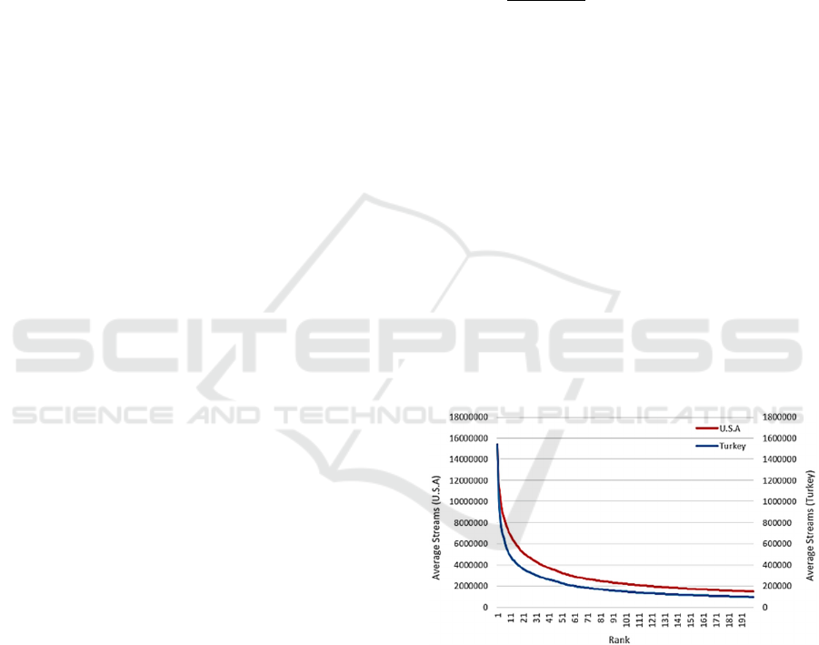
The first notable difference between the two

datasets is the total number of streams. Since the

number of Spotify users are higher in the U.S., it is

not unexpected. In Turkey, decrease in the song

stream when rank increase is sharper. This shows that

higher ranked songs have distinctly higher stream

values than the lower ranked songs. In Figure 2 we

plot the average number of streams for each rank (1-

200) for both countries.

Figure 2: Comparison of the number of average streams

over weeks.

Figure 3 shows the total weekly streams of the

Turkish songs “Heyecanı Yok”, ”Beni Sen İnandır”

and “Let Me Down Slowly” until the last appearance

in the Top 200 charts. Each of the three songs have

followed different patterns for 2 years which shows

us that appearing in the charts longer does not imply

the higher number of streams and vice versa.

A Longitudinal Model for Song Popularity Prediction

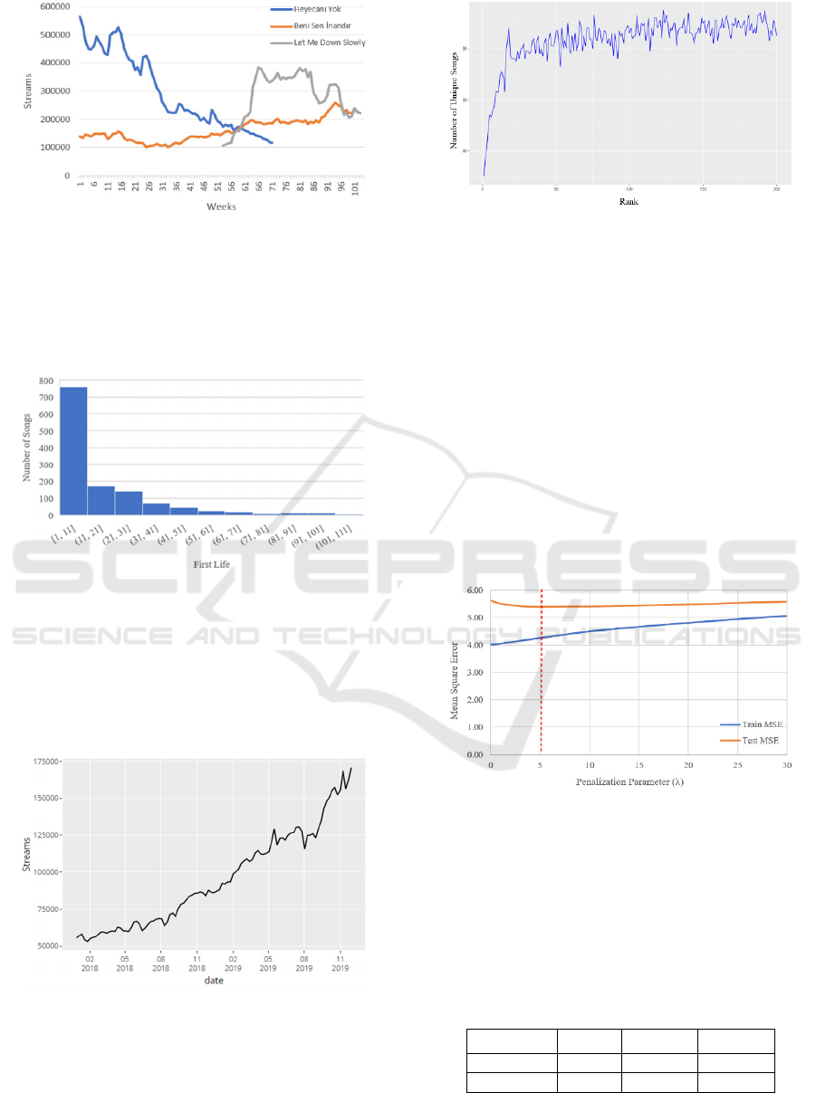
Figure 3: Comparison of the streams of 3 songs in Turkey's

charts.

Each song has different first lives in the charts

which shows its number of weeks that it shows up in

the charts after first release. In Figure 4, histogram of

the first lives in the Turkey is shown.

Figure 4: Histogram of the first lives of the songs in Turkey.

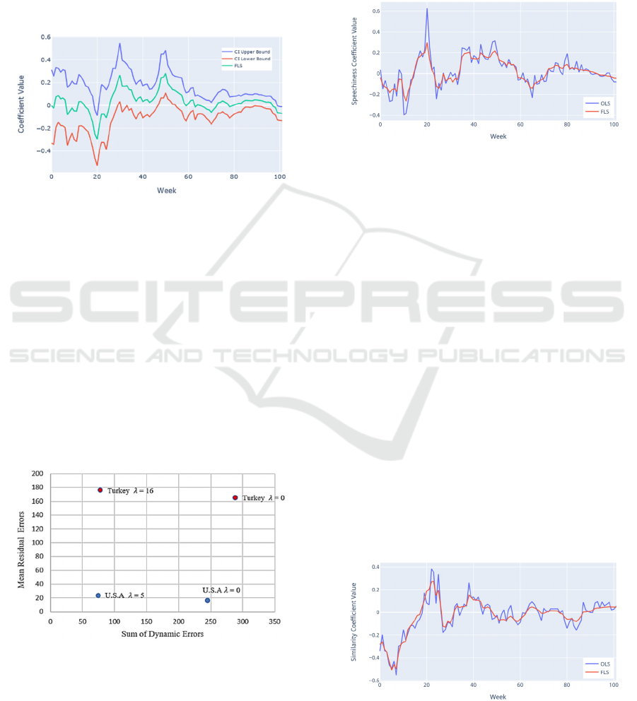
During the two years, the total number of

streamed songs has increased due to the increase in

the number of users and the spread of music

streaming platforms. This increase can be seen even

in the change of the stream of the 200

songs over 2

years in Figure 5.

Figure 5: Number of streams for 200th song in Turkey.

Each 200 rank have been shared by different

number of unique songs in 2 years. Figure 6 shows

that the appearing in the higher ranks could be

achievable for a couple of successful songs.

Figure 6: Number of unique songs in each rank.

4.2 Computational Results

We solved FLS model on a PC with 8 GB RAM and

Intel Core i7-8550U 1.80 GHz processors using

CPLEX 12.8 solver on Python 3.7. Before starting to

solve the model, we decided the value of the

penalization parameter. To determine the

penalization parameter 𝜆, we applied 5-fold cross

validation by fitting the regression model for 10

weeks of data with different 𝜆 values. We found the

best 𝜆 value both for Turkey and the U.S. Figure 7

shows the cross-validation results for train and test

sets for the U.S dataset and the selected value for the

penalization parameter. Selected values for Turkey

and the U.S. datasets are 16 and 5, respectively.

Figure 7: Change of the dynamic and residual errors with

the change of the penalization parameter.

Each run of the model takes 4.51 second in

average and it takes 11297 minutes for completing

2500 bootstrap samples for Turkey’s dataset. In

Detailed statistics for computational times can be

seen in Table 1.

Table 1: Run time statistics (seconds) of the optimization

model across bootstrap samples.

Country Min Median Max

Turke

3.31 4.51 15.68

U.S. 3.94 6.01 16.48

DATA 2021 - 10th International Conference on Data Science, Technology and Applications

100

As mentioned in the Section 3, we used bootstrapping

to generate confidence bounds for the regression

parameters. The number of bootstrap samples is

selected to be 2500. These samples were generated

with Monte Carlo cross validation method by

selecting 120 samples from the common songs that

appears in both the previous and the next weeks’

charts. In Figure 8, we show the change of the 90%

confidence bounds and the estimations generated by

bootstrapping.

Figure 8: FLS estimate of acousticness variable in Turkey

with bootstrap 90% confidence intervals.

FLS method creates smoother transitions between

consecutive weeks’ coefficients by penalizing the

dynamic error in the objective function. However,

this causes a worse fit for the overall model and the

accuracy. Cross-validation allowed us to choose the

best lambda values for the datasets so that we can

achieve smooth shifts between the weeks while

keeping the regression errors as small as possible. In

Figure 9 the change of the objective function value

with the OLS and FLS for both datasets can be seen.

Dynamic errors decreases with the increase of the 𝜆

so that we had smooth transitions between weeks

while increase in the SSE is small.

Figure 9: Train and test errors of the cross-validation sets.

There are some obvious patterns occurred in the

coefficient changes of the Turkey’s regression

outputs. Especially in the 20

week of our dataset and

the following weeks, there are significant rises and

falls in the various coefficients. In 2018, the rap/trap

music rush started in Turkey. Even the old rap songs

such as “Neyim Var ki” released in 2004, appeared

and survived in the top 200 charts with the increasing

popularity of this genre. Typical characteristics of the

rap/trap songs are the high speechiness and low

energy. Figure 10 shows the changes in the regression

coefficients of the speechiness variable.

Figure 10: OLS and FLS estimates of Turkey's

"Speechiness" coefficient.

Another coefficient that shows us a similar

outcome is “Similarity” which is generated by

calculating the cosine similarity of the songs in a

week. Around the 20

weeks, increase of the

similarity coefficient shows a similar pattern with the

other rap related characteristics. Figure 11 shows the

FLS output of the similarity coefficient over time.

We also wanted the compare the popularity of

local and foreign artists, so we separated the

popularity variable for Turkey’s dataset as mentioned

in the Section 4.1. However, we could not detect

different patterns on these two variables.

In the timeline of the FLS coefficients of the U.S.,

“valence” seems to have an apparent temporal

behaviour variable. Valence is a measure from 0.0 to

1.0 that describes the musical positiveness of a track.

Higher valence means happier songs. At the end of

the years, coefficient of the valence increases and

then decreases in a couple of weeks. As the Christmas

time arrives, people tend to listen old songs related

the holiday. These Christmas songs are happier songs

thus they have higher valence.

Figure 11: OLS and FLS estimates of Turkey’s “Similarity

coefficient.

A Longitudinal Model for Song Popularity Prediction

101

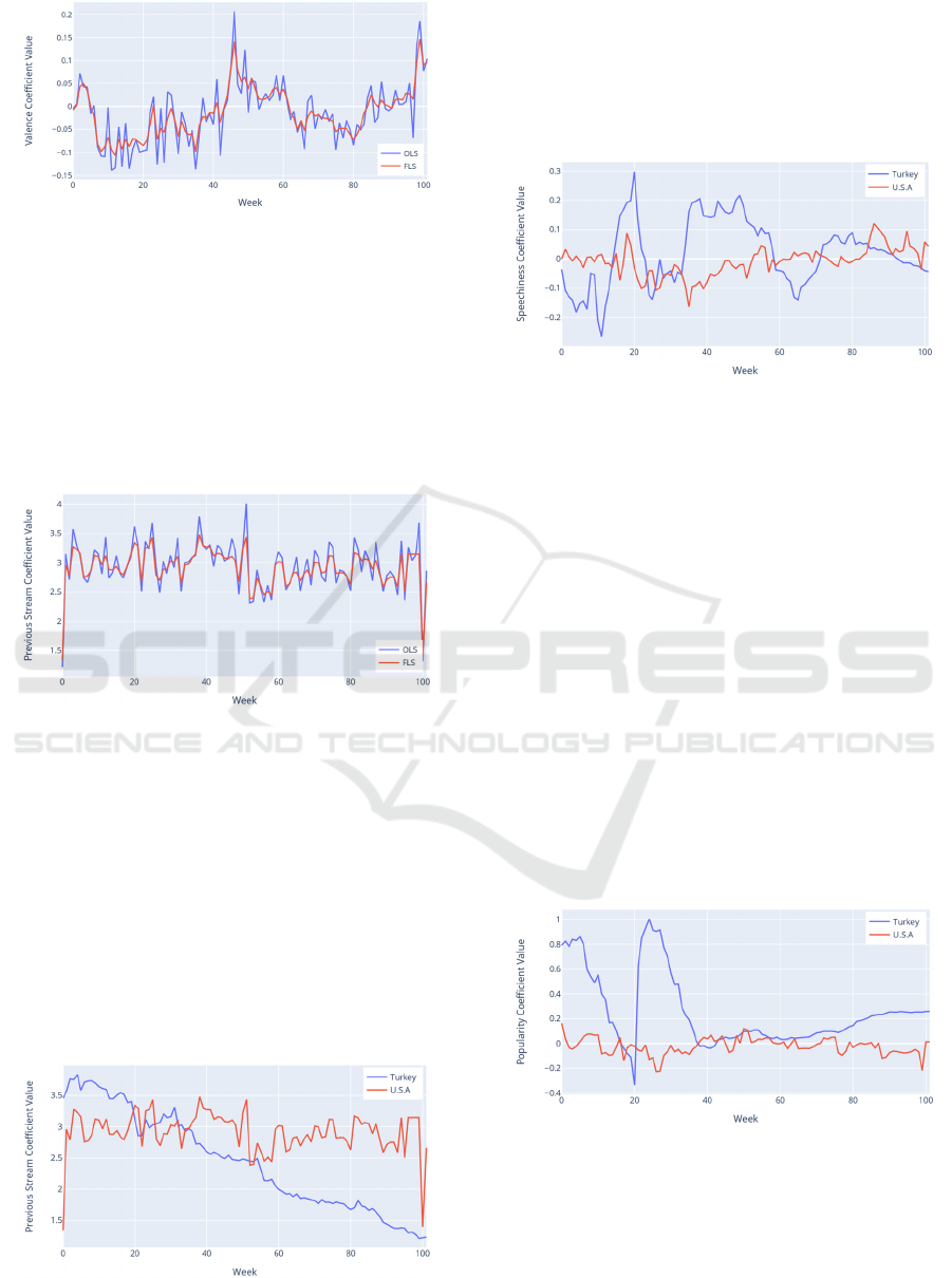
Figure 12: OLS and FLS estimates of the U.S.’s “Valence”

coefficient.

Another similar pattern is observed in the

coefficients of the U.S. is the “Previous Stream”. As

mentioned before, the “Previous Stream” variable is

generated using a song’s previous week stream.

Negative peaks in the beginning of 2018 and at the

end of the 2019 may show the relationship between

the increasing popularity of the Christmas songs

which has less previous streams than the new songs.

Figure 13: OLS and FLS estimates of the U.S.’s “Previous

Stream” coefficient.

Another important motivation in this study is to

reveal cross-cultural differences of the musical

attributes. We expected that similar or different

patterns may be observable in the regression

coefficients of Turkey and the U.S. The coefficient

of the “Previous Stream” variable follows a different

pattern. As we mentioned before, coefficient value of

the “Previous Stream” is decreasing with the

Christmas in the U.S. It does not follow a similar

pattern in Turkey’s results. Coefficients of the

variable have a decreasing pattern.

Figure 14: Comparison of two countries’ FLS coefficient of

the “Previous Stream” variable.

Speechiness is another variable that has an

obvious pattern in Turkey’s results which represents

the rap songs’ increasing popularity However, we can

not see such pattern change in the U.S.’s speechiness

variable. In Figure 15, country comparison

speechiness coefficients are shown.

Figure 15: Comparison of two countries’ FLS coefficient of

the “Speechiness” variable.

Popularity is one of the features that Spotify

calculates for each artist. Higher popularity means

being most popular. When we compare the popularity

coefficients of Turkey and the U.S., it is apparent that

the artist popularity affects the music stream in a

different manner for these countries. In Turkey,

Popularity had a positive effect on the song streams

in the first quarter and this effect decreased in

following 20 weeks. After a sudden change in 20

week, artist popularity became positively effective for

the songs in Turkey. For the rest of the weeks,

popularity does not follow a strict pattern which may

show us; with the rise of the new trends/artists its

effect decreases over time. In the U.S. artist

popularity is not effective on a song’s as Turkey’s

2019 pattern. In Figure 16 comparison of the FLS

coefficients for the popularity coefficients of two

countries are shown.

Figure 16: Comparison of two countries’ FLS coefficient of

the “Popularity” variable.

As mentioned before, the similarity metric has

followed a pattern that may highlight the shifts in

Turkey’s music listening habits with the rap music

trend. In the U.S., coefficients of the “Similarity”

metric seems to be ineffective on the song streams

DATA 2021 - 10th International Conference on Data Science, Technology and Applications

102

which shows that the influence of the songs with

similar acoustic attributes did not affect songs’

number of streams. Comparison of the “Similarity”

coefficients of the countries is shown in Figure 17.

Figure 17: Comparison of two countries’ FLS coefficient of

the “Similarity” variable.

Another variable that we generated in addition to

Spotify’s acoustic features is “Release Date”. We

expected to see different effects of the song recency on

the song streams. Release dates of the songs are

discretized as equal probability intervals as mentioned

in Section 4.1. The comparison of the coefficients of

the newest songs is shown in Figure 18. In Turkey, the

new songs have a positive coefficient during 2018.

However, song recency became ineffective in 2019. In

the U.S., there are no significant changes in the

coefficient except the year's ends.

Figure 18: Comparison of two countries’ FLS coefficient of

the “The Newest Releases” variable.

As result, we observed that the music listening

habits in Turkey change more than in the U.S. These

changes can be seen in the coefficient changes over

time more clearly. It can be said that political and

economic dynamics in Turkey may affect the social

influence on music listening habits differently.

5 CONCLUSIONS AND FUTURE

WORKS

In this paper, we proposed an application of the FLS

method on music data to analyze shifts in music taste

and popularity over different countries. We used

quadratic programming with bootstrapping to solve

the model and generate the confidence bounds for the

regression coefficients of the features. FLS method

allows us to smoothen the coefficient changes in time

so that the changes in the coefficients are reflected

realistically. Our findings show that the acoustic

features of the songs may have an effect on the song's

popularity and there may be obvious patterns in the

regression coefficients so that we can observe the

shifts in the music tastes.

As future work, one should analyze/compare

more countries’ musical tastes with the help of new

information and methods. Since our work consists of

2 countries’ data in 2 years, it can be extended with

more data from different countries and length of

periods. Our methodology is also able to be

diversified with a new constant parameter time series

regression model and a smoothing method applied to

the OLS coefficients for comparing the methods with

the FLS.

REFERENCES

Al-Beitawi, Z., Salehan, M., and Zhang, S. (2020). What

makes a song trend? Cluster analysis of musical

attributes for Spotify top trending songs. Journal of

Marketing Development and Competitiveness, 14(3):

79-91.

Efron, B. (1992). Bootstrap methods: another look at the

jackknife. In Breakthroughs in statistics (pp. 569-593).

Springer, New York, NY.

Box, G. E., and Cox, D. R. (1964). An analysis of

transformations. Journal of the Royal Statistical

Society: Series B (Methodological), 26(2): 211-243.

Buda, A., and Jarynowski, A. (2015). Exploring patterns in

European singles charts. In 2015 Second European

Network Intelligence Conference (pp. 135-139). IEEE.

Herremans, D., Martens, D., and Sörensen, K. (2014).

Dance hit song prediction. Journal of New Music

Research, 43(3): 291-302.

Kalaba, R., and Tesfatsion, L. (1989). Time-varying linear

regression via flexible least squares. Computers &

Mathematics with Applications, 17(8-9): 1215-1245.

LeBlanc, A., Jin, Y. C., Chen-Hafteck, L., de Jesus

Oliviera, A., Oosthuysen, S., and Tafuri, J. (2000).

Tempo preferences of young listeners in Brazil, China,

Italy, South Africa, and the United States. Bulletin of

the Council for Research in Music Education, 97-102.

Lütkepohl, H., and Herwartz, H. (1996). Specification of

varying coefficient time series models via generalized

flexible least squares. Journal of Econometrics: 70(1),

261-290.

Mulligan, M. (2020, June 23). Music subscriber market

shares Q1 2020. Midia Research. https://www.midia

research.com/blog/music-subscriber-market-shares-

q1-2020

A Longitudinal Model for Song Popularity Prediction

103

Ni, Y., Santos-Rodriguez, R., Mcvicar, M., and De Bie, T.

(2011, December). Hit song science once again a

science. In 4th International Workshop on Machine

Learning and Music.

Pınarbaşı, F. (2019). Demystifying musical preferences at

Turkish music market through audio features of Spotify

charts. Turkish Journal of Marketing, 4(3): 264-279.

Rentfrow, P. J., and Gosling, S. D. (2003). The do re mi's

of everyday life: the structure and personality correlates

of music preferences. Journal of personality and social

psychology, 84(6): 1236.

Sciandra, M., and Spera, I. C. (2020). A model-based

approach to Spotify data analysis: A Beta GLMM.

Journal of Applied Statistics, 1-16.

Schedl, M., and Hauger, D. (2012, April). Mining

microblogs to infer music artist similarity and cultural

listening patterns. In Proceedings of the 21st

International Conference on World Wide Web (pp. 877-

886).

Spotify (2021, March 16). Spotify company info.

https://newsroom.spotify.com/company-info/

Stone, J. (2020, October 6). The State of the Music Industry

in 2020. Toptal Finance Blog. https://www.

toptal.com/finance/market-research-analysts/state-of-

music-industry

Suh, B. J. (2019). International Music Preferences:

An Analysis of the Determinants of Song Popularity

on Spotify for the US, Norway, Taiwan, Ecuador,

and Costa Rica. (Claremont McKenna College

Senior Theses). https://scholarship.claremont.edu/

cmc_theses/2271

Spotify for Developers. (2014, March 6). Spotify.

https://developer.spotify.com/community/news/2014/0

3/06/echo-nest-joins-spotify/

Wood, B. D. (2000). Weak theories and parameter

instability: Using flexible least squares to take time

varying relationships seriously. American Journal of

Political Science, 603-618.

Yadati, K., Liem, C. C., Larson, M., and Hanjalic, A. (2017,

June). On the automatic identification of music for

common activities. In Proceedings of the 2017 ACM on

international conference on multimedia retrieval (pp.

192-200).

Yeo, I. K., and Johnson, R. A. (2000). A new family of

power transformations to improve normality or

symmetry. Biometrika, 87(4): 954-959.

DATA 2021 - 10th International Conference on Data Science, Technology and Applications

104