Mixed Software/Hardware based Neural Network Learning Acceleration
Abdelkader Ghis
1,2 a
, Kamel Smiri
2,4 b
and Abderezzak Jemai
3 c
1
University of Tunis El Manar, Tunis, 1068, Tunisia
2
Laboratory of SERCOM, University of Carthage/Polytechnic School of Tunisia, 2078, La Marsa, Tunisia
3
Carthage University, Tunisia Polytechnic School, SERCOM-Lab., INSAT, 1080, Tunis, Tunisia
4
University of Manouba/ISAMM, Manouba, 2010, Tunisia
Keywords:
Neural Network, Learning, Back-propagation, Data Partitioning, Neural Network Distribution.
Abstract:
Neural Network Learning is a persistent optimization problem due to its complexity and its size that increase
considerably with system size. Different optimization approaches has been introduced to overcome the mem-
ory occupation and time consumption of neural networks learning. However, with the development of mod-
ern systems that are more and more scalable with a complex nature, the existing solutions in literature need
to be updated to respond to the recent changes in modern systems. For this reason, we propose a mixed
software/hardware optimization approach for neural network learning acceleration. The proposed approach
combines software improvement and hardware distribution where data are partitioned in a way that avoid the
problem of local convergence. The weights are updated in a manner that overcome the latency problem and
learning process is distributed over multiple processing units to minimize time consumption. The proposed
approach is tested and validated by exhaustive simulations.
1 INTRODUCTION
Neural network learning is a time consuming task
(Ghosh et al., 2018), especially in case of large
amounts of data, when thousands of stimulus should
be trained by the network. Computing power of the
built-in neural network devices would be insufficient,
which leads to the hardware enhancement or cloud
services use. This enhancement is studied by time and
passed by the improvement of computational power
of devices. Recent fields are moving from hardware
improvement to software design and acceleration to
face the latency and connectivity coasts (Al-Fuqaha
et al., 2015). Distributing the neural networks infer-
ence and learning is one of the most studied tech-
niques for the artificial intelligence neural network
(Lin et al., 2017). Neural network learning is the main
task in neural network conception, by which the neu-
ral network weights, bias, layer and connections are
adjusted. Regarding its complexity while facing huge
amount of data and large neural network sizes, this
task consumes energy, processing power and requires
a
https://orcid.org/0000-0002-2668-1663
b
https://orcid.org/0000-0001-8739-3887
c
https://orcid.org/0000-0003-4033-2969
a large time interval. Several software and hardware
implementation for neural network learning are pro-
posed in the goal of task acceleration, i.e., time and
energy optimization by distributing the learning pro-
cess and paralleling different tasks.The concept of
distributing the artificial neural network is not new.
Since 1995 R.J. Howlett & D.H.Lawrence proposed
the distribution of the neural network learning over
multiple computers in the goal of reducing the learn-
ing time complexity. The proposed neural network
in which the input layer forward a copy of the input
data over the multiple feed-forward neural network
blocs. And an output layers with build in winner-
takes-all algorithm. An approach which approved its
efficiency in term of time complexity. This work is
also optimized by an approach of changeable num-
ber of blocs depending on the accessible processors
(Adamiec-Wojcik et al., 2005). Bontak.G & Young
Geun.K (Gu et al., 2019) proposed a framework for
distributed deep neural network training with het-
erogeneous computing platform, the training require-
ment are estimated by performing some training task
to select by the end the best cluster of heterogeneous
platforms for the training. Surat.T & H.T Kung (Teer-
apittayanon et al., 2017a) distributed a deep neural
network over cloud, edge and devices, the distribu-
Ghis, A., Smiri, K. and Jemai, A.
Mixed Software/Hardware based Neural Network Learning Acceleration.
DOI: 10.5220/0010606104170425
In Proceedings of the 16th International Conference on Software Technologies (ICSOFT 2021), pages 417-425
ISBN: 978-989-758-523-4
Copyright
c
 2021 by SCITEPRESS – Science and Technology Publications, Lda. All rights reserved
417

tion is made bay implementing some exit points after
every level end i.e. an exit point after the end of the
neural network portion implemented in the device, if
the result is satisfying the process ends, else the pro-
cessing moves to upper level. this distribution is made
for the neural network inference. Chen. J & Philip.
S.Y. (Chen et al., 2018) proposed an architecture deal-
ing with the problem of distributing the neural net-
work and the training data set. Incremental data parti-
tioning and allocation was proposed and also a global
weight updating was proposed. This last is dealing
with the problem of the heterogeneity of the different
components of the target system. In the goal of pass-
ing over the problem of the deference between pro-
vided computing power of the different components;
which has an impact on the time response of each
one.The strategy is proposed in a way that eliminating
the waiting part of the process and updating weight
after every received weight update. The experiments
of such technique showed that the proposed method-
ology improves the training time and the accuracy of
the CNN. Henry .S & Venkatesan.M (Selvaraj et al.,
2002) implemented a large neural network using de-
composition. Instead of implementing one large neu-
ral network, this last was decomposed functionally
into sub-networks ended final sub-network which col-
lects all other sub-networks outputs. The second tech-
nique was the data decomposition for less complexity
and faster learning. While studying existing method-
ologies in literature, we investigated the weakness of
some of these approaches when dealing with data and
weights update.
The data decomposition proposed in (Gu et al.,
2019) (Adamiec-Wojcik et al., 2005),(Chen et al.,
2018), (Selvaraj et al., 2002) is based on functional
dependencies which may be an accuracy enhancer,
but in terms of time it is very costly. First, the data de-
composition is an added task before the training starts,
this task delays the training process depending on the
data-set volume. Second, in case of parallel neural
network learning and sub-data-set allocation for each
task, delays the weight convergences i.e., each task
which is executed in parallel converges its weights
only for the data portion allocated for the given neu-
ral network portion, it may be very efficient for the
given sub-data, but for the complete data is complex
and need more training time.
The back-propagation algorithms in (Gu et al.,
2019), (Adamiec-Wojcik et al., 2005), (Chen et al.,
2018), (Selvaraj et al., 2002), (Teerapittayanon et al.,
2017b), are tasks which can be executed in parallel.
However, these tasks are executed in the same pro-
cessing unit. This double execution within the same
processing unit delays the optimal weights search pro-
cess.
In the goal of enhancing the learning time and
overcoming all the mentioned points above we pro-
pose a technique which combine two approaches,
software improvement and hardware distribution, in
which data are partitioned in a manner that overcomes
the problem of local convergence. We propose also a
weights update technique for latency problem, and a
distributed learning approach over multiple process-
ing units.
2 PRELIMINARIES
This section provides the concepts of artificial neural
networks such concepts, architecture and principles.
2.1 Artificial Neural Network
Artificial neural network (ANN) is one of the most
promising machine learning implementation (Yoon,
2019). It is widely used in different real life
domains, covering sales(Aritonang and Sihombing,
2019) and price estimation, security and attack con-
trolling (Yoon, 2019), healthcare domain and epi-
demic controlling (Ahmed et al., 2020; Le et al.,
2021; Kiran et al., 2021a), demotic including smart
homes and quality control in industry 4.0, disasters
estimations, weather estimation and even the inter-
national exchanges. Neural Networks are used to
address nonlinear regression analysis problems(Ly
et al., 2021). It has been proved that a neural network
with only one hidden layer can simulate very complex
nonlinear functions (Bishop, 2006).ANN mimics the
cognitive function which is traditionally associated to
the human brain (Yoon, 2019). Neural Networks pro-
vides also computational models designed to solve a
specific problem (Razafimandimby et al., 2016).
2.2 ANN Architecture
Artificial neural network architecture consists of mul-
tiple processing layers, where each layer consists of
multiple processing units, known as neurons (Saleem
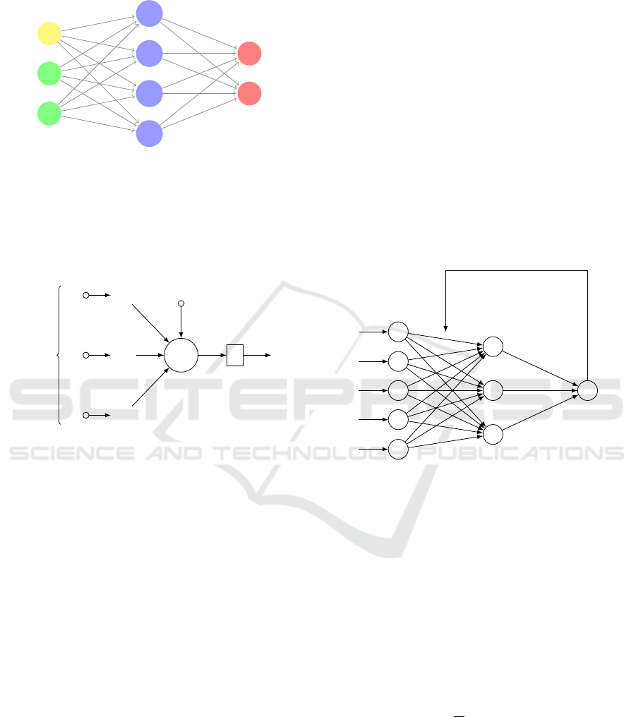
and Chishti, 2019). Figure 1 presents the simple neu-
ral network architecture (Kiran et al., 2021b).
A simple neural network is composed of input
layer, hidden layer and an output layer. Inputs di-
rected to a central unit called neuron for an activation
function (the processing function) ended by output as
described. The number of neurons in the input layer
depends on the features number of incoming data, the
number of output neurons depends on the use case of
the neural network, .i.e ” in the case of classification,
ICSOFT 2021 - 16th International Conference on Software Technologies
418

x
0
x
1
x
2
Input
layer
h
(1)
1
h
(1)
2
h
(1)
3
h
(1)
4
Hidden
layer
ˆy
1
ˆy
2
Output
layer
Figure 1: Simple Neural Network Architecture.
the number of neurons in the output layer is the num-
ber of classes or cluster in output”, where the num-
ber of neurons in hidden layers changes according to
the learning technique. Each computational unit or
x
2
w
2
Σ
f
Activate
function
y
Output
x
1
w
1
x
3
w
3
Weights
Bias
b
Inputs
Figure 2: One Neuron Internal Processing.
so called neuron has a weighted inputs, bias and an
activation function, the built in function then is given
with the following equation:
out put = f (
I
∑
i
w
i
x
i
+ b) (1)
where
• x
i
: the inputs
• w
i
: connections’ weights
• b : the bias
• I : inputs’ number of the given neuron
• f : the activation function
One neuron is connected to previous neurons from
previous layer, those connections are weighted i.e.
each connection has an associated weight, by which
the previous neurons output is multiplied. An read-
justment value called bias is added to the sum of the
weighted inputs. This formula is called activation
function, where the second function called transfer
function which has different variations (Sigmoid, Sig-
moid linear unit, Identity..) for the output normaliza-
tion. this process continues until the output layer is
reached.
2.3 Back Propagation
The back propagation algorithm is a supervised ma-
chine learning method for efficient training of the neu-
ral network (Liu and Baiocchi, 2016). The main fea-
ture in this algorithm is its iterative, recursive and
efficient method for updating weights. The back
propagation algorithm is one of the most used algo-
rithms when dealing with classification and regres-
sion neural networks. Figure 3 illustrates how the
back-propagation moves from the end of the architec-
ture (output layer) to the beginning (input layer).
Input
layer
Hidden
layer
Output
layer
Input 1
Input 2
Input 3
Input 4
Input 5
error
Error back propagation
Figure 3: Back Propagation.
The back propagation algorithm can be applied
to train all connections weights of multi-perceptrons
neural network(Sapna et al., 2012). The term back-
propagation describes how the gradual computation
of nonlinear neural network is performed (Teerapit-
tayanon et al., 2017a). The gradient descent func-
tion is one of the most used in neural network back-
propagation training. Weights with the minimum er-
ror function are the solution for the learning problem.
Back-propagation based on the gradient descent uses
the gradient of e Mean Squared Error (MSE)(Kolbusz
et al., 2019) demonstrated in the following equation:
MSE =
1
N
N
∑
i=1
(y
i,ex
− y
i,out
)
2
(2)
where the one weight modification is given by
w
k+1
= w
k
− γg(w
k
) (3)
• y
i,ex
: the desired output
• y
i,out
: the real output
• N : data features number
Mixed Software/Hardware based Neural Network Learning Acceleration
419

• w
k+1
: updated weight
• w
k
: the current weight
• γ : learning rate
The process and direction of modification is illus-
trated in Figure 4.
y
(l)
i
y
(l+1)
1
.
.
.
y
(l+1)
m
(l+1)
δ
(l+1)
1
δ
(l+1)
m
(l+1)
Figure 4: Back Propagation.
Here δ
(l+1)
1
corresponds to the errors that are prop-
agated back from layer (l+1) to layer (l).Once it is
evaluated for the outputs, it can be propagated in
backward.
3 PROPOSED NEURAL
NETWORK LEARNING
APPROACH
In this section, we present our methodology by de-
scribing data partitioning process, neural network dis-
tribution process, weights update and communication.
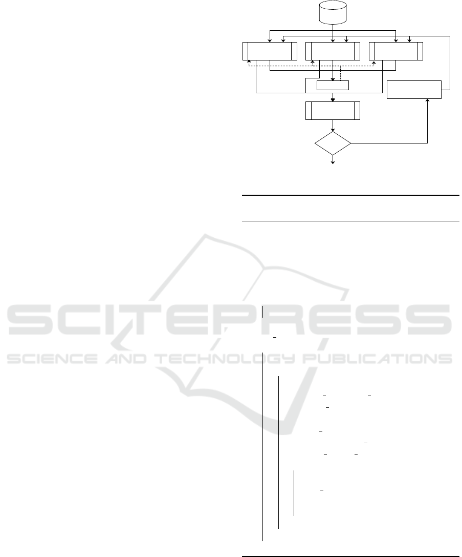
data
set
<
>
=
GLOBAL PARAMETERS
forward units
backward unit
back-propagation
unit
Min error
index
comparison
ANN
ANN
ANN
ANN
data allocation
parameters allocation
error transfer
index transfer
back-propagation
parameters transfer
updated
weights transfer
Figure 5: General Approach Description.
Figure 5 gives a general description of the target
processing scheme. It shows how the neural network
is distributed, how data are allocated and how weights
are calculated and updated.
3.1 Formalization
This subsection formulates the proposed methodol-
ogy for neural network learning acceleration.
3.1.1 Data Partitioning
Our aim is to work on complete neural network over
multiple processing units, with a full neural network
copied in each unit. Regarding the data partitioning
proposed in (Ghosh et al., 2018) and (Atzori et al.,
2010), functional decomposition results an distributed
neural network composed of multiple functional sub-
networks. The second one which works on the whole
neural network, data decomposition causes the prob-
lem of local convergence, where every copied neural
network in each block converges its weights depend-
ing on the data portion allocated for the processing
block, and not the whole data-set. This last delays
the processing and global weights convergence. Our
technique is to keep the raw structure of the data-set.
Furthermore, instead of dividing it in functional por-
tion, we shuffle the order of stimulus in the data-set
and allocate one stimulus randomly for each incom-
ing call from the processing unit.
For a given data-set of N stimulus, the access to
each stimulus consumes θT units of time, and the al-
location of each one to the target subset consumes α
T unit of time. Finally the stimulus transfer from the
data-set to the processing unit memory needs γT unit
of time. This process of distributing the data-set as
discussed in the previous works in literature, called
distribution time Dt is important and delays the be-
ginning of learning process by Dt unit of time. This
last is calculated as following in equation:
Dt = N ∗ (θT + αT + γT ) (4)
Our approach is to distribute this distribution time to
immediately start the learning process and to not de-
laying it with the Dt time, i.e., the first epoch of the
learning process stars after the first memory access
and instead of waiting for the whole distribution pro-
cess time, each processing unit starts the learning after
its access to the memory and import the stimulus.The
waiting time Wt becomes as follows:
Wt = (θT + γT ) (5)
where the θT the time needed to access to the data in
the memory and γT is the importation time of the data
to the processing unit.
The other benefit of our approach is the memory re-
quirement needed. Instead of duplicating the data-
set size over the processing units, only small memory
storage is needed to save the imported stimulus.
ICSOFT 2021 - 16th International Conference on Software Technologies
420

3.1.2 Neural Network Distribution
With the goal of accelerating the learning process, we
duplicate the complete neural network structure over
the provided processing units which is considered as
sub-werker units (Eddine et al., 2020) to work on the
weights in parallel, then, for a given E number of
epochs, and T the time needed to process all stimu-
lus of the data-set, the total time to process the whole
data-set for all the epochs is given by
ET = (ExT) (6)
For a given Pn the number of provided processing
units, the processing time will be in the average of
+/ − PT = (ET /Pn) (7)
which is based on the heterogeneity of the processing
blocks. The processing time is reduced depending on
the number of processing units.
In each node or processing unit, and for time ac-
celeration, the back-propagation process will be inde-
pendent, which means either dividing the processing
unit into two blocks or allocating two processing units
for each neural network copy. The foreword pass for
the output calculation will be done in the first block,
where the back-propagation will be executed in the
second one. The first block of the processing will
be free and up to process new neural network output,
when the second block is working on weights calcu-
lation and update in parallel.
For the given data-set of N stimulus, with a
one processing unit, and for E number of epochs.
In case of feed-forward neural network with back-
propagation algorithm. the process is divided into two
steps.The forward pass to calculate the neural network
output, and the back-forward pass to readjust the neu-
ral network weights. The forward pass consumes φFt
unit of time and the back-forward pass consumes ϕBt
units of time. The learning time is described by the
following equation:
Lt = E ∗ (N ∗ (φFt + ϕBt)) (8)
To accelerate the learning process, we distribute the
learning process by multiplying the processing units
by which, the learning time will be reduces depending
on the processing units count. For a Np the number of
processing units, the learning time formula becomes
as follows:
Lt = (E ∗ (N ∗ (φFt + ϕBt)))/Np (9)
The processing units can be heterogeneous,then, the
learning time will be in the average of Lt because of
the difference of calculation speed and occupation of
the processing units.
3.1.3 Weights Update
Weights update is an independent process in an inde-
pendent processing unit. Every forward unit submits
its error which is the difference between the desired
output and the calculated output the comparison unit.
The purpose of the-back propagation is to minimize
the error and maximize the accuracy. In this stage one
forward unit parameters and results are chosen with
the minimum error is selected. The comparison unit
notifies the selected forward unit by its index. This
forward nit transfers its parameters and result to the
back-propagation unit, in which the back-propagation
process starts. And while working on the weight up-
date the forward units are freed, then it starts a new
process on new data with the old weights till the
weights are updated. Once the back-propagation pro-
cess is done, the resulting weights are submitted to the
parameter unit which is also an independent unit. In
this stage a master-slave program is applied, and it al-
locates weights to each forward unit with new process
on a new data. Waiting for all units to finish the calcu-
lation and update the global weight matrix is critical
and cause a delay of ∆T the waiting time of all units
to finch calculation. This ∆T is added to the learning
time Lt and delays it. the replication algorithms with
the immediate update is adopted to surpass this chal-
lenge and optimise the learning time and reduce it by
∆T. The learning time formula becomes as follows:
Lt = ((E ∗ (N ∗ (φFt + ϕBt)))/Np) − ∆T (10)
3.1.4 Communication
Communicating the learning data to the processing
unit in the previous works, by dividing the data-set
to sub-data-sets and transferring it, is very consuming
task. First, the data replicated results a double mem-
ory occupation with the same stored data. Second,
transferring the sub-set occupies the communication
way and becomes very dense, which means complex.
keeping the raw form of the data set, and communi-
cating only a required data to the requester unit is one
of our techniques to reduce the communication cost in
term of time and memory occupation. For deep neu-
ral networks, weight matrix are extremely large con-
taining thousands of values. Matrix transfer is a com-
munication cost consuming, there-fore, energy con-
suming. Especially for our approach, where differ-
ent blocks are transferring their matrix to the unique
weights unit, by which, the communication cost in-
creases. The key here is not to transfer the whole
weight matrix coming from the different processing
units (forward units), but the quadratic error value in-
stead, which gives a feedback about the pertinence
Mixed Software/Hardware based Neural Network Learning Acceleration
421

of the weights based on the processed data (stimu-
lus) .Once the processing unit is selected as mini-
mum eroor, it will be the one and only unit to trans-
fer its local weights and forward results to the back-
propagation unit. Paralleling the two function of data
transfer and learning processes is a time gainer. Com-
pared to the previous sequential methods of executing
the data transfer followed by learning process. Instead
of focusing on whole data transfer, our system trans-
fers only the required data which means reducing the
waiting time to start the process of learning as men-
tioned in equation 10.
The transfer of the local calculated weight matrix
of M weight, from Np processing units to back-
propagation unit, consumes Mt unit of time per ma-
trix and Mb unit of bandwidth. For the Np processing
units, the transfer time Tt equation is given by
Tt = Np ∗(Mt) (11)
Transferring only one value which is the error in-stead
of the complete matrix is time and bandwidth gainer,
and it reduces the transfer time to be as follows:
Tt = (Np ∗(1ut)) + Npu +Mt (12)
The 1ut is one unit of time needed to transfer accu-
racy from one processing unit, Npu is the units of
time needed to select the minimum error plus the time
of transferring the selected matrix Mt . Our method-
ology is a time gainer. First, it parallelizes the data
transfer which reduces the processing time, by which
the learning task starts earlier instead of waiting un-
til the transfer ends. Second, parellizing the back-
propagation with the forward process eliminates the
waiting time double functions in one processing unit.
Finally, it reduces the communication cost in term of
time and energy while it transfers only simple values
and one matrix instead of thousands of weights val-
ues.
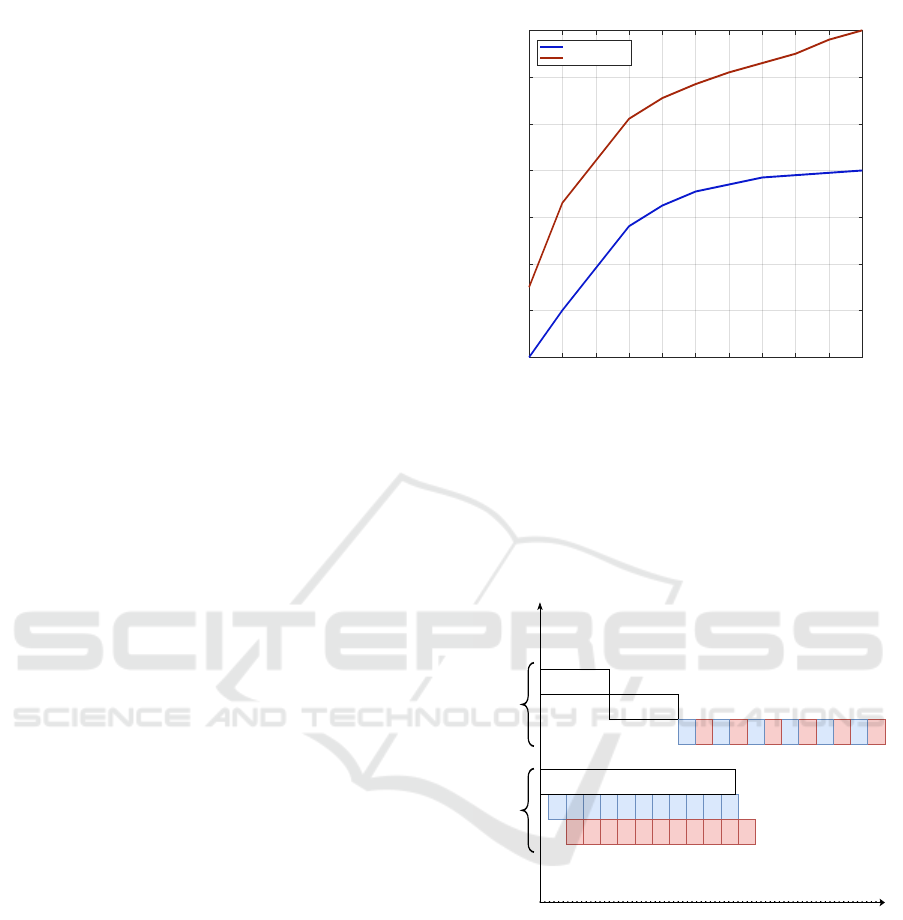
Figure 6 summarizes our proposed formulation.
3.2 Implementation
This subsection implements the proposed methodol-
ogy with the following algorithm.
This algorithm summarizes the methodology
course. After the initialisation of the data-set and allo-
cating the available processing units ( five processing
units in our case) and the choice of the neural network
architecture, these parameters are taken as inputs to
our system. The back-propagation process starts after
the forward task is done, for this reason, the firs iter-
ation is made independently from the loop, by which
we calculate the first three (03) outputs of the three
forward
unit
forward
unit
forward
unit
data
set
min(error)
backward
unit
end
epochs
parameters
unit
data allocation
error transfer
index notification
parameters transfer
updated weights allocation
NO
YES
updated weights submission
final weights
Figure 6: General Approach Flow Description.
Algorithm 1: Distributed Parallel Neural Net-
work Learning.
1 Input: input variables &NN Architecture
2 Output: optimal weightsand bias
initialization
3 Let Pr = { P1,P2,P3,P4,P5}
4 Let D = { d1, d2, d3, d4,..., PN} : N data
count
5 for k ← 1 to 3 do
6 Error ← allocate(dk toPk);
7 end
8 min index = minimum(Error);
9 while i < E do
10 Paralleling { P1, P2, P3, P4, P5;
11 for j ← 4 to N do
12 parameter ←
import f rom(min index);
weights update ←
allocate(parameter to P4);
//back propagation unit
allocate(weights updateto P5);
13 allocate global weights(P5 toP1, P2,P3);
14 for k ← 1 to 3 do
15 Error < −allocate(d jk toPk);
16 min index = minimum(Error);
17 j ← j + 3; // increment data index
by 3 steps
18 end
19 end
20 end
allocated processing units for the forward task. Once
the output is calculated and parameters are selected
based on the error function, the epochs loop starts.
Paralleling all allocated processing unit for our sys-
tem, we give the selected parameters to the backward
processing unit for the weight update, in the same
ICSOFT 2021 - 16th International Conference on Software Technologies
422

time, we allocate new data to the three processing
units with the old weights looking for parameters with
minimum error function. The backward output which
is the updated weights is sent to the parameter units,
this last uses the server-slave algorithms to modify pa-
rameters in the three first processing units. Depending
on the number of epochs, we loop this task till the end
of epochs. The output of our system is a fast learned
neural network with optimal weight and bias.
4 APPROACH SIMULATION
This section presents the simulation results of our pro-
posed methodology.
4.1 Simulation Setup
In the purpose of making sense of our methodology, a
simulation was conducted on an intel(R) Core(TM)i7-
8550U HP-CPU with 16GB RAM, using Visual Stu-
dio 2019 C# neural network script. The choice of
c# language is justified with the objective of easily
embed it on a programmable card. A 4-50-3 fully
connected neural network architecture is used, which
means four neurons in the input layer, fifty neurons
in the hidden layer, and three neurons in the output
layer. the dataset used in our learning process is ran-
domly generated data of 4 features inputs and 3 fea-
tures output, adequately to our neural network archi-
tecture. For the comparison stage, the same neural
network was implemented with the same language.
For the data partitioning task, the K-means algorithm
was implemented with the number of clusters equal to
the number of available processing units.
4.2 Simulation Results
This subsection demonstrates the obtained results of
the proposed approach.
4.2.1 Data Access
In our approach, the key to minimize the learning time
is to parallelize the learning and the data access.
Figure 7 shows the impact of this parallelization
and how it reduces the learning time process. The key
in data allocation is to provide one data to the comput-
ing unit instead of allocating a full cluster by which
the computing task starts earlier and is reduced from
Tl to Te. Compared to the implemented literature ap-
proach, our approach is time gainer by avoiding the
partitioning task as shown in the curve.
0 500 1000 1500 2000 2500 3000 3500 4000 4500 5000
Number of Epochs
0
1000
2000
3000
4000
5000
6000
7000
Time (ms)
Distributed DNN
Proposed Approach
Figure 7: Learning Time.
4.2.2 Parallelized Processing
In this stage, we simulate the distribution of the neu-
ral network over different computing blocks by paral-
lelizing the scripts that should be embedded on the
computing blocks, as shown in figure 8. For each
data decomposition
data allocation
data allocation
FFFFFFFFFFF
FFFFFF
BpBpBpBp
BpBpBpBpBpBp
BpBpBpBpBpBpBp
Time
literature
approach
proposed
approach
Figure 8: Parallelism impact.
block, one data is allocated to compute the neural net-
work output, for a given three units as defined in our
simulation. The second part of parallelism is the sep-
aration between the backward and forward task. By
this parallelism (distributing in hardware blocks), the
browsing time of the whole data-set is reduced and
divided by 2 due to the backward task isolation. An-
other time gainer key in our approach as shown in fig-
ure 8 compared to the time needed to process data by
literature approaches.
Mixed Software/Hardware based Neural Network Learning Acceleration
423

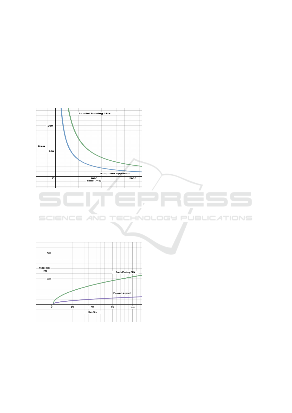
4.2.3 Impact on Error Function
The learning error calculated during the system ex-
ecution shown in figure 9 for both, our proposed
methodology and literature methodologies . Our
methodology shows how it is better than the other
studied approaches, due to the selection process of the
minimum error, by which it works on the parameters
with minimum errors and enhance to get closer to the
optimal weights.
Figure 9: Errors.
the accuracy is enhanced by 0.07 % due to the error
minimization process.
4.2.4 General Cases Impact
Figure 10 shows the impact of the data size change
on our approach. The figure shows how our approach
Figure 10: Waiting Time.
is always a time gainer compared to other approaches
in term of data size and even processing units. The
delay time is related to the time of transferring one
data compared to other technique, which consumes
more time to split data and allocates the data portions
every time the data set get bigger.
5 CONCLUSION
In this paper, we propose an optimization for neural
network learning acceleration. This optimization is
based on software and hardware enhancement to re-
duce learning time and facilitate data access. We pro-
pose a smart data access method which avoid the de-
lay and waiting time to start the learning process. In
addition, we distribute the learning process over mul-
tiple processing units that work independently. More-
over, we isolated the back-propagation task and se-
lect only the minimum error parameters to update
weights. Results show that our methodology is a time
gainer and it reduce the learning process time by more
than two times. The data size change doesn’t have an
impact on our methodology due to the smart access
we implemented. The accuracy is enhanced due to the
selection technique.Regarding the studied approaches
in the literature, our approach is a time gainer and
overcomes the weakness points denoted above.
REFERENCES
Adamiec-Wojcik, I., Obrocki, K., and Warwas, K. (2005).
Distributed neural network used in control of brake
torque distribution. In 2005 IEEE Intelligent Data Ac-
quisition and Advanced Computing Systems: Technol-
ogy and Applications, pages 116–119. IEEE.
Ahmed, I., Ahmad, A., and Jeon, G. (2020). An iot
based deep learning framework for early assessment
of covid-19. IEEE Internet of Things Journal.
Al-Fuqaha, A., Guizani, M., Mohammadi, M., Aledhari,
M., and Ayyash, M. (2015). Internet of things: A
survey on enabling technologies, protocols, and ap-
plications. IEEE communications surveys & tutorials,
17(4):2347–2376.
Aritonang, M. and Sihombing, D. J. C. (2019). An applica-
tion of backpropagation neural network for sales fore-
casting rice miling unit. In 2019 International Con-
ference of Computer Science and Information Tech-
nology (ICoSNIKOM), pages 1–4. IEEE.
Atzori, L., Iera, A., and Morabito, G. (2010). The internet of
things: A survey. Computer networks, 54(15):2787–
2805.
Bishop, C. M. (2006). Pattern recognition and machine
learning. springer.
Chen, J., Li, K., Bilal, K., Li, K., Philip, S. Y., et al. (2018).
A bi-layered parallel training architecture for large-
scale convolutional neural networks. IEEE transac-
tions on parallel and distributed systems, 30(5):965–
976.
ICSOFT 2021 - 16th International Conference on Software Technologies
424

Eddine, C. C., Salem, M. O. B., Khalgui, M., Kahloul, L.,
and Ougouti, N. S. (2020). On the improvement of
r-tncess verification using distributed cloud-based ar-
chitecture.
Ghosh, A., Chakraborty, D., and Law, A. (2018). Artificial
intelligence in internet of things. CAAI Transactions
on Intelligence Technology, 3(4):208–218.
Gu, B., Kong, J., Munir, A., and Kim, Y. G. (2019). A
framework for distributed deep neural network train-
ing with heterogeneous computing platforms. In 2019
IEEE 25th International Conference on Parallel and
Distributed Systems (ICPADS), pages 430–437. IEEE.
Kiran, K. S., Azman, M., Nandu, E., and Prakash, S. S.
(2021a). Real-time detection and prediction of heart
diseases from ecg data using neural networks. In
Proceedings of International Conference on Recent
Trends in Machine Learning, IoT, Smart Cities and
Applications, pages 93–119. Springer.
Kiran, K. S., Azman, M., Nandu, E., and Prakash, S. S.
(2021b). Real-time detection and prediction of heart
diseases from ecg data using neural networks. In
Proceedings of International Conference on Recent
Trends in Machine Learning, IoT, Smart Cities and
Applications, pages 93–119. Springer.
Kolbusz, J., Rozycki, P., Lysenko, O., and Wilamowski,
B. M. (2019). Error back propagation algorithm with
adaptive learning rate. In 2019 International Confer-
ence on Information and Digital Technologies (IDT),
pages 216–222.
Le, D.-N., Parvathy, V. S., Gupta, D., Khanna, A., Ro-
drigues, J. J., and Shankar, K. (2021). Iot enabled
depthwise separable convolution neural network with
deep support vector machine for covid-19 diagnosis
and classification. International Journal of Machine
Learning and Cybernetics, pages 1–14.
Lin, J., Yu, W., Zhang, N., Yang, X., Zhang, H., and Zhao,
W. (2017). A survey on internet of things: Archi-
tecture, enabling technologies, security and privacy,
and applications. IEEE Internet of Things Journal,
4(5):1125–1142.
Liu, X. and Baiocchi, O. (2016). A comparison of the def-
initions for smart sensors, smart objects and things in
iot. In 2016 IEEE 7th Annual Information Technol-
ogy, Electronics and Mobile Communication Confer-
ence (IEMCON), pages 1–4. IEEE.
Ly, H.-B., Nguyen, T.-A., and Pham, B. T. (2021). Estima-
tion of soil cohesion using machine learning method:
A random forest approach. Advances in Civil Engi-
neering, 2021.
Razafimandimby, C., Loscri, V., and Vegni, A. M. (2016).
A neural network and iot based scheme for perfor-
mance assessment in internet of robotic things. In
2016 IEEE first international conference on internet-
of-things design and implementation (IoTDI), pages
241–246. IEEE.
Saleem, T. J. and Chishti, M. A. (2019). Deep learning for
internet of things data analytics. Procedia computer
science, 163:381–390.
Sapna, S., Tamilarasi, A., Kumar, M. P., et al. (2012).
Backpropagation learning algorithm based on leven-
berg marquardt algorithm. Comp Sci Inform Technol
(CS and IT), 2:393–398.
Selvaraj, H., Niewiadomski, H., Buciak, P., Pleban, M., Sa-
piecha, P., Luba, T., and Muthukumar, V. (2002). Im-
plementation of large neural networks using decom-
position.
Teerapittayanon, S., McDanel, B., and Kung, H.-T. (2017a).
Distributed deep neural networks over the cloud, the
edge and end devices. In 2017 IEEE 37th Interna-
tional Conference on Distributed Computing Systems
(ICDCS), pages 328–339. IEEE.
Teerapittayanon, S., McDanel, B., and Kung, H.-T. (2017b).
Distributed deep neural networks over the cloud, the
edge and end devices. In 2017 IEEE 37th Interna-
tional Conference on Distributed Computing Systems
(ICDCS), pages 328–339. IEEE.
Yoon, J. (2019). Using a deep-learning approach for smart
iot network packet analysis. In 2019 IEEE European
Symposium on Security and Privacy Workshops (Eu-
roS PW), pages 291–299.
Yoon, J. (2019). Using a deep-learning approach for smart
iot network packet analysis. In 2019 IEEE European
Symposium on Security and Privacy Workshops (Eu-
roS&PW), pages 291–299. IEEE.
Mixed Software/Hardware based Neural Network Learning Acceleration
425