Extending DEAP with Active Sampling for Evolutionary Supervised

Learning

Sana Ben Hamida

1 a

and Ghita Benjelloun

Paris Dauphine University, PSL Research University, CNRS, UMR[7243], LAMSADE, 75016 Paris, France

Paris Dauphine University, PSL Research University, 75016 Paris, France

Keywords:

Genetic Programming, DEAP, Active Learning, Random Sampling, Weighted Sampling, Occupancy

Detection, Pulsar Detection.

Abstract:

Complexity, variety and large sizes of data bases make the Knowledge extraction a difﬁcult task for supervised

machine learning techniques. It is important to provide these techniques additional tools to improve their

efﬁciency when dealing with such data. A promising strategy is to reduce the size of the training sample

seen by the learner and to change it regularly along the learning process. Such strategy known as active

learning, is suitable for iterative learning algorithms such as Evolutionary Algorithms. This paper presents

some sampling techniques for active learning and how they can be applied in a hierarchical way. Then, it details

how these techniques could be implemented into DEAP, a Python framework for Evolutionary Algorithms. A

comparative study demonstrates how active learning improve the evolutionary learning on two data bases for

detecting pulsars and occupancy in buildings.

1 INTRODUCTION

Learning from complex, large and unbalanced

databases is a major issue for most of the current data

mining and machine learning algorithms. More pow-

erful knowledge discovery techniques are needed to

deal with the related challenges. Evolutionary Data

Mining tools, such as Genetic Programming (GP), are

powerful meta-heuristics with an empirically proven

efﬁciency on complex machine learning problems.

Thus, the use of evolutionary data mining procedures

becomes a hot trend. Thanks to their global search

in the solution space, evolutionary computation tech-

niques help in the information retrieval from a volu-

minous pool of data in a better way compared to tradi-

tional retrieval techniques. Thus, they are part of the

promising tools to discover insights within the grow-

ing complexity and volume of available data. How-

ever, as all machine learning techniques, GP needs

some extensions to improve its efﬁciency when learn-

ing from large, complex or unbalanced datasets. This

paper investigates the use of active learning paradigm

to scale evolutionary data mining techniques to com-

plex data sets.

Active learning (Atlas et al., 1990; Cohn et al.,

1994) is a learning paradigm based on active sam-

https://orcid.org/0000-0003-4202-613X

pling techniques. The goal of any sampling approach

is to extract subsets from the original training set in

order to reduce the size or to handle some anomalies

such unbalanced classes . With active learning, subset

sampling is applied regularly along the training pro-

cess in order to change frequently the examples seen

by the algorithm. Subset selection could be done ran-

domly or according to a given strategy such data dif-

ﬁculty based strategy (Gathercole and Ross, 1997) or

data topology based strategy (Lasarczyk et al., 2004;

Hmida et al., 2016b). Active learning is successfully

implemented with iterative learning algorithm such as

evolutionary data mining methods.

This work outlines how we extended an existing

GP implementation with active sampling techniques

using three strategies: random selection, balanced se-

lection and weighted selection based on age and dif-

ﬁculty of exemplars. Random and weighted sampling

methods are applied on a balanced set extracted from

the training data base in order to handle the classes

unbalance problem. We also investigate the applica-

tion of multi-level sampling using different sampling

techniques on a hierarchical way. These strategies are

implemented on a Python framework for evolution-

ary algorithms, DEAP. They are applied to solve two

classiﬁcation problems: pulsar classiﬁcation and oc-

cupancy detection in buildings.

574

Ben Hamida, S. and Benjelloun, G.

Extending DEAP with Active Sampling for Evolutionary Supervised Learning.

DOI: 10.5220/0010604605740582

In Proceedings of the 16th International Conference on Software Technologies (ICSOFT 2021), pages 574-582

ISBN: 978-989-758-523-4

This paper is organized as follows. First we re-

mind brieﬂy the evolutionary loop, the GP engine

and the their implementation over the Python frame-

work DEAP. Section 3 explains the active learning

paradigm and details the sampling techniques im-

plemented for this work: Random Sampling (RSS),

Balanced sampling (SBS) and Weighted Sampling

(DSS). Details about the implementation of these

techniques over DEAP are given in section 4. Sec-

tion 5 summarizes the classiﬁcation problems for the

experimental study. The main results are summarized

and discussed in section 5.2 before the conclusion.

2 BACKGROUND

2.1 EAs: A Brief Overview

Evolutionary algorithms (EAs) are zero

order opti-

mization methods based on a random search of the

parameter space by a population of optimizers under-

going ”evolutionary pressure” based on an analogy

with Darwinian selection of species EAs are based on

the evolution of a population of solutions X

(individ-

uals), where X

a candidate solution to the problem.

Each solution X

is evaluated to give some measure

of its performance (ﬁtness). The minimisation of this

measure during the process drive the evolution of the

population. At each generation, a set of new individu-

als (offspring) are generated by selecting the more ﬁt

individuals. These offspring undergo transformations

(alter step) by means of ”genetic” operators : muta-

tion (perturbation of a solution) and crossover (com-

bination of solutions) (Petrowski and Ben-Hamida,

2017). A new population is then formed by a stochas-

tic selection among offspring proportionally to their

ﬁtness.

2.2 Genetic Programming

Genetic Programming (GP) is a dynamic tree based

representation for EAs. It is applied to evolve com-

plex objects such as sequential sub-programs or lin-

ear functions. GP is considered as the evolutionary

technique having the widest range of domain appli-

cation. Thanks to its great ﬂexibility, GP is able to

solve different classes of machine learning problems

such as data classiﬁcation and symbolic regression. In

this paper, GP is used to solve two classiﬁcation tasks

described in section 5.

GP respects the same EAs main steps as EA

as described above. The GP population is an en-

semble of dynamic syntax trees composed of a

set of leaves, called terminals and a set of nodes,

called non-terminals. The non-terminal set may in-

clude arithmetic operations, mathematical functions,

boolean operations, conditional operators (such as

If-Then-Else), functions causing iteration (such as

Do-Until),etc. The terminals are, typically, variable

atoms (i.e, representing the inputs) or constant atoms

or functions with no explicit arguments. To evolve

the GP population, speciﬁc initialization and varia-

tion operators are needed. DEAP framework, de-

scribed below, proposes a great variety of mutation

and crossover operators ready to use.

GP has shown its great potential when applied

to supervised learning, especially classiﬁcation prob-

lems. GP evolves a population of classiﬁers (genetic

programs) by means of genetic operators through gen-

erations. The general GP loop for supervised learn-

ing is illustrated in Fig 1. Two data sets (at least) are

needed: the training set and the test set. The training

set is used by the algorithm along the learning pro-

cess to evaluate the evolved models (steps 1 and 4 in

Fig 1). The test set is used to assess the accuracy of

the ﬁnal models (step 6 in Fig 1). The two sets must

be independent such as all test instances are unknown

from the learner. Each pattern is evaluated according

to its corresponding error across the test set. For a

classiﬁcation problem, the error might be estimated

according to the number of misclassiﬁed cases.

2.3 DEAP

DEAP (or Distributed Evolutionary Algorithm in

Python) (Fortin et al., 2012) is a Python framework

released in 2012 at the Vision and Numerical Systems

Laboratory (LVSN) at the Laval university of Canada.

It is freely available and is presented as a rapid proto-

typing and testing framework. It implements several

EA: Genetic Algorithms, Evolution Strategies (ES)

and Genetic Programming.

The core architecture of DEAP is built around dif-

ferent components that deﬁne the speciﬁc parts of

what is an evolutionary algorithm and what is an evo-

lutionary learning loop (Fig 1). DEAP’s core is com-

posed of three modules: base, creator, and tools. The

base module contains objects and data structures fre-

quently used in Evolutionary Computation that are

not already implemented in the Python standard li-

braries.

To implement functional programming paradigm

used by GP, DEAP propose different data structure

such as lists and trees. For each data structure, a set

of crossover and mutation operator is available. For

this work, we choose the basic GP trees. The non

terminal set, DEAP propose a collection of unary and

binary arithmetic operators, a collection of mathemat-

Extending DEAP with Active Sampling for Evolutionary Supervised Learning

575

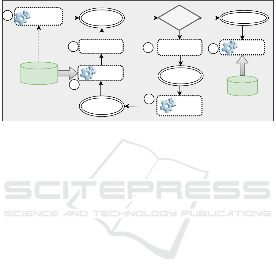
Current

Population

Parents

Parents +

offspring

Stop? Final population

Training

sample

Variation

operators

Fitness

evaluation

Initialization

Evaluation

Parental

selection

Survival

Selection

Validation

Test

sample

Yes

Figure 1: Genetic Learning Evolutionary loop. Steps 2,3 and 5 concern the traditional EA loop. Steps 1 and 4 need training

data sample. Model validation in step 6 needs test data sample.

ical functions such as logarithmic functions and a set

of logic operators.

3 ACTIVE LEARNING

With Evolutionary data mining techniques, it is pos-

sible to train all models on a single subset S . The

subset S is then used to evaluate all individuals (mod-

els) throughout an evolutionary run. This sampling

approach known as the Static Sampling. If any sam-

pling technique is called by the learner to change the

training set along the evolution, then it is the Active

Learning paradigm that is applied.

Active Learning (Atlas et al., 1990; Cohn et al.,

1994) could be deﬁned as:

‘any form of learning in which the learning

program has some control over the inputs on

which it trains.’

Active learning is implemented essentially with

active sampling techniques. The goal of any sampling

approach is to reduce the original size of the train-

ing set, and thus the computational cost, and enhance

the learner performance. Sampling training data set

has been ﬁrst used to boost the learning process and

to avoid over-ﬁtting (Iba, 1999). Later, it was in-

troduced for Genetic learners as a strategy for han-

dling large input databases. With the increasing size

of available training datasets, this practice is widely

used.

With active sampling, the training subset is

changed periodically across the learning process. We

distinguish one-level sampling methods using a sin-

gle selection strategy and multi-level sampling (hier-

archical sampling) methods using multiple selection

strategies associated in a hierarchical way.

3.1 One-level Active Sampling

One-level sampling methods use a single selection

strategy based on dynamic criteria, such random se-

lection, weighted selection, incremental selection,

etc. Records in the training subset S are selected be-

fore the application of the genetic operators each η

(η ≥ 1) generations. When η = 1, the population is

evaluated on a different data subset each generation

and the sampling approach is called generation-wise.

If the main goal of the sampling technique is the

reduction of the training ﬁtness cases for the eval-

uation step, the subset selection can be performed

randomly, as described in the following (subsec-

tion 3.1.2). However, if the sampling method has

an additional purpose (avoiding over-ﬁtting, improve

learning quality, handling imbalanced data, etc), it

needs a speciﬁc record selection strategy. It is the

case of several sampling approaches in the litera-

ture. For example, the Topology Based Sampling

method (Lasarczyk et al., 2004; Hmida et al., 2016a)

studies relationship between ﬁtness cases in the data

base in order to avoid to select similar ﬁtness cases

in the same training subset. Its objective is to maxi-

mize the generalization ability of the applied machine

learning technique. To overcome imbalance in the

original data base, a series of balanced sampling tech-

niques are proposed in (Hunt et al., 2010). For a clas-

ICSOFT 2021 - 16th International Conference on Software Technologies

576

siﬁcation problem, these techniques aim to improve

the classiﬁers accuracy by correcting the data imbal-

ance within majority and minority class instances in

the selected subset. For this work, we are interesting

on the balanced, random and weighted sampling.

3.1.1 Balanced Sampling (SBS)

The main purpose of balanced sampling is to over-

come imbalance in the original data sets. The well

known techniques in this category are those proposed

by Hun et al. (Hunt et al., 2010) aiming to im-

prove classiﬁers accuracy by correcting the original

dataset imbalance within majority and minority class

instances. Some of these methods are based on the

minority class size and thus reduce the number of in-

stances. In this paper, we focus on the Static Balanced

Sampling (SBS). SBS is an active sampling method

that selects cases with uniform probability from each

class without replacement until obtaining a balanced

subset. This subset contains an equal number of ma-

jority and minority class instances of the desired size.

3.1.2 Random Sampling (RSS)

The simplest method to choose ﬁtness cases (data

record) to build the training sample S is random. This

stochastic selection helps to reduce any bias within

the full dataset on evolution. Random Subset Selec-

tion (RSS) is the ﬁrst implementation given by Gath-

ercole et al. (Gathercole and Ross, 1994). In RSS,

at each generation g, the probability of selecting any

case i is equal to P

(g) such that :

∀i : 1 ≤ i ≤ T

, P

(g) =

. (1)

where T

is the size of the full dataset B and T

is the target subset size. The sampled subset has a

ﬂuctuating size around T

3.1.3 Weighted Sampling (DSS)

Weighted Sampling techniques have two objectives:

(i) focus the algorithm abilities on difﬁcult cases, i.e.

ﬁtness cases frequently unsolved by the best solu-

tions,

(ii) check ﬁtness cases that have not been looked at

for several generations.

The ﬁrst algorithm in this category is Dynamic Subset

Selection (DSS) (Gathercole and Ross, 1997; Gath-

ercole, 1998). This algorithm is intended to preserve

training set consistency while alleviating its size by

keeping only the difﬁcult cases with ones not selected

for several generations.

To each dataset record is assigned a difﬁculty de-

gree D

(g) and an age A

(g) starting with 0 at ﬁrst

generation and updated at every generation. The dif-

ﬁculty is incremented for each misclassiﬁcation and

reset to 0 if the ﬁtness case is solved. The age is equal

to the number of generations since last selection, so it

is incremented when the ﬁtness case has not been se-

lected and reset to 0 otherwise. The resulting weight

W of the i

ﬁtness case is calculated as follows:

∀i : 1 ≤ i ≤ T

, W

(g) = D

(g)

+ A

(g)

. (2)

where d is the difﬁculty exponent and a is the age

exponent. The selection probability of a record i is

biased by its weight W

such that:

∀i : 1 ≤ i ≤ T, P

(g) =

(g) ∗ S

∑

j=1

(g)

. (3)

DSS needs three parameters to be tuned: difﬁculty

exponent, age exponent and target size.

3.2 Multi-level Active Sampling

Multi-level sampling or hierarchical sampling com-

bines several sampling algorithms applied in different

levels. Its objective is to deal with large data sets that

do not ﬁt in the memory, and simultaneously provide

the opportunity to ﬁnd solutions with a greater gen-

eralization ability. The data subset selections at each

level are independent (Fig 2).

The hierarchical sampling was ﬁrst experimented

for an intrusion detection problem in (Robert Curry,

2004). RSS and DSS was combined to implement two

level sampling methods: RSS-RSS and RSS-DSS.

Authors proposed also in (Curry et al., 2007) the BB-

DSS techniques where a balanced sampling is applied

in the ﬁrst level. The aim is to handle classes’ unbal-

ance by generating balanced blocks from the starting

data base. These blocks are then used as input for

the second level sampling. The same approaches are

also experimented in (Hmida et al., 2018) to solve the

Higgs Boson classiﬁcations problem.

Figure 2: Multi-level Sampling for Evolutionary Machine

Learning. Level 1 and 2 sampling are iterated within the

Evolutionary loop.

Extending DEAP with Active Sampling for Evolutionary Supervised Learning

577

3.3 Implemented Schema

In this work, four sampling schema are implemented

that are variants from the one-level and multi-level

sampling methods described above:

• 2L-RSS: two level random sampling. At level 0,

balanced bloks are created with a same ratio for

each class using the SBS technique. At level 1, the

random sampling is applied on the current block.

• 2L-DSS: as for 2L-RSS, the weighted sampling at

level 1 is applied on the balanced blocks created

at level 0.

• 3L-RSS-DSS: It is a 3 level sampling technique

based on the 2L-RSS and extended with a third

level where a weighted sampling is applied on the

subset given by RSS.

• 3L-RSS-RSS: It respects the same steps as 3L-

RSS-DSS. However, the random selection is ap-

plied twice, at level 1 and 2.

To implement these techniques, additional parameters

are needed to deﬁne the block size, the training set

size and the intermediate training set size for the three

level sampling. Otherwise, the sampling frequency

for each level is also an input parameter to be deﬁned.

4 ENABLING ACTIVE

SAMPLING OVER DEAP

This section details how DEAP is extended with the

different sampling techniques proposed in this work.

First, the whole train set is loaded in a pandas data

frame that is used as an input argument for SBS to

create Blocks (Fig 2 - Level 0).

The code of the SBS and RSS sampling methods

used in this work is given in Fig 3. For the DSS

algorithm, the training data is extended with 3 addi-

tional columns : Age (A), Difﬁculty (D) and Weight

(W) that are updated each generation according to the

equation 2. The parameters d and a are set to 1 and

3.5 as in (Hmida et al., 2016b). However, the selec-

tion step is slightly modiﬁed. Before selecting a new

train set from the input sample, the data frame is di-

vided into two blocks (one for each class) in order to

use both balance and weight criteria for the sampling

method.

4.1 Extending DEAP with 2 Level

Active Sampling

As introduced in section 3, all active sampling tech-

niques are applied on a balanced data (BBtrain) hav-

ing BBSize records. It is created at level 0 of each

sampling algorithm according to the following proce-

dure. This code is then integrated in the GP loop.

#each g_level0 generations

if g(\% g_level0)==0

BBtrain=SBS([trainSet,BBSize)

To implement the level 1 sampling, according to

the conﬁguration, one method from RSS, SBS and

DSS is applied on the balanced block BBtrain each

level1 generations.

#each g_level1 generations

if g(\% g_level1)==0

#RSS or SBS or DSS

finalSet=BBtrain.RSS(setSize)

4.2 Extending DEAP with 3 Level

Active Sampling

With the three-level sampling, an additional sampling

step is performed just after the level 1 such as the ﬁnal

training sample is selected from an intermediate data

set (intermSet) generated from BBtrain randomly or

with a balanced sampling.

BBtrain −→ IntermSet −→ ﬁnalSet

(BBsize) (IntSetSize) (setSize)

The aim of this additional step is to train GP popu-

lation on a smaller sample in order to further reduce

the GP computational cost and the DSS sampling cost

when it applied. At each generation, the population of

classiﬁers is evaluated on the f inalSet sample.

5 APPLICATION

To assess the efﬁciency of the active sampling for su-

pervised learning over DEAP, we selected two data

sets with different characteristics and difﬁculties.

ODS Data Set for Occupancy Detection in

Buildings:

Occupancy detection in an ofﬁce room uses data

from light, temperature, humidity and CO

sensors

(Candanedo and Feldheim, 2016a). Ground-truth oc-

cupancy was obtained from time stamped pictures

that were taken every minute. The Occupancy is

the response variable indicated with 0 and 1 (occu-

pied/empty). Occupancy detection using the ODS

ICSOFT 2021 - 16th International Conference on Software Technologies

578

def RSS(InputSet,setSize):

OutputSet=InputSet.sample(setSize) #select randomly a sample of setsize instances

return OutputSet

def SBS(InputSet,setSize):

# Create two random sub-samples from each class

OutputSet_class0=InputSet[InputSet.iloc[:,0]==0].sample(setSize//2)

OutputSet_class1=InputSet[InputSet.iloc[:,0]==1].sample(setSize//2)

# contact the two sub-samples

OutputSet=pd.concat(OutputSet_class0,OutputSet_class1)

return OutputSet

Figure 3: DEAP implementing RSS and SBS sampling methods.

def DSS(InputSet,setSize):

#update weights of all exemplars

InputSet.iloc[:,-1] = InputSet.iloc[:,-2]**d + InputSet.iloc[:,-3]**a

InputSet_class0=InputSet[InputSet.iloc[:,0]==0]

InputSet_class1=InputSet[InputSet.iloc[:,0]==1]

IntputSet_class0.sort_values(by = 'W', ascending = False)

IntputSet_class1.sort_values(by = 'W', ascending = False)

OutputSet = pd.concat(IntputSet_class0.iloc[:setSize//2],

IntputSet_class1.iloc[:setsize//2])

return OutputSet

Figure 4: DEAP implementing DSS sampling method.

data set is a medium difﬁculty classiﬁcation problem

that has been solved with different machine learning

techniques. The classiﬁcation accuracy might reach

99% with some techniques such as SVM (Elkhoukhi

et al., 2018). The purpose of using this data in the

present work is to study the effect of adding one-

level and multi-level sampling techniques to a power-

ful machine learning technique such that GP to solve

a non difﬁcult classiﬁcation problem.

HTRU Data Set for Pulsar Detection:

Pulsars are a rare type of Neutron star that produce

radio emission detectable on Earth. They are of con-

siderable scientiﬁc interest as probes of space-time,

the inter-stellar medium, and states of matter (Lyon

et al., 2016a). As pulsars rotate, their emission beam

sweeps across the sky, and when this crosses our line

of sight, produces a detectable pattern of broadband

radio emission. As pulsars rotate rapidly, this pat-

tern repeats periodically. Thus pulsar search involves

looking for periodic radio signals in observational

data.

Machine learning classiﬁers are applied for pulsar

detection since 2010. A state of the art is published in

(Wang et al., 2019). The ﬁrst data base made publicly

available contains 22 features. Lyon et al. (Lyon et al.,

2016b) demonstrated that some features may be sub-

optimal for machine learning classiﬁer and proposed

the HTRU data set with 8 features. It is this second

data base studied in the present work.

The HTRU data set contains 16,259 spurious ex-

amples caused by RFI/noise (the majority negative

class), and 1,639 real pulsar examples . These ex-

amples have all been checked by human annotators.

Classiﬁcation machine learning tools are used to au-

tomatically label pulsar candidates to facilitate rapid

analysis. The ability of machine learning technique

applied for pulsar detection is proved in several works

(Azhari et al., 2020).

Table 1: Data sets information.

Data Attributes Set Negative Train

Set size examples data

ODS 5 Real Values 8143 6414 6000

HTRU 8 Real Values 17898 16259 14000

5.1 GP Settings and Performance

Measures

GP are trained on the both data sets using parameters

summarized in Table 2.

For each data set, ﬁve series of tests are per-

formed. For each series, a different conﬁguration is

Extending DEAP with Active Sampling for Evolutionary Supervised Learning

579

Table 2: GP parameters.

Parameter Value

Population size 200

Generations number 150

Tournament size 4

Crossover probability 0.5

Mutation probability 0.2

GP Tree depth 3

Fitness Classiﬁcation error

Selection operator Selection by tournament

Crossover operator Point crossover

applied according to the sampling strategy. For each

data set, GP is extended with one of the following

conﬁgurations:

• No Sampling : GP is run without active learning.

The whole data set is seen by each classiﬁer at

each generation.

• Two Level Sampling: GP is extended with a two

level sampling using SBS a the ﬁrst level and RSS

(2L-RSS) or DSS (2L-DSS) at the second level.

• Three Level Sampling: GP is extended with a

three level sampling using the same hierarchy as

Two Level Sampling and adding RSS (3L-RSS-

RSS) or DSS (3L-RSS-DSS) at the last level.

Ten runs with different seeds are performed for each

conﬁguration. By the end of each run, the confusion

matrix of best classiﬁer according to the test set is

recorded and its accuracy and recall are computed ac-

cording to the following formula.

Accuracy =

True Positives + True Negatives

Total examples

. (4)

Recall =

True Positives

True Positives + False Negatives

. (5)

where True Positives and True Negatives are the

numbers of exemplars correctly classiﬁed in respec-

tively class 1 and 0, False Positives and False Nega-

tives are the numbers of exemplars incorrectly classi-

ﬁed.

Additional parameters are set for the sampling

techniques to deﬁne the size of the training set and

the sampling frequency at each level. Their values are

summarized in Table 3.

Experiments are performed on an Intel i7 (4

Core) workstation with 16GB RAM running under

Windows 64-bit Operating System.

5.2 Results and Discussion

The main objective of an active sampling technique is

to improve the performance of the learning algorithm

according to either the quality of the obtained results

by maximizing the generalization ability or accord-

ing to the computational cost by minimizing the run

time. Both measures are recorded for each run. Ta-

ble 4 and 5 summarize the best and average accuracy,

the best computing time and the best recall for each

conﬁguration.

Three main observations can be deduced from the

experimental results. First, introducing a sampling

technique to GP helps reducing the training cost up to

10 times, and often with improved performance. Fig 5

shows the relative time saving according to the com-

puting time of the standard GP without sampling. It is

near 90% for the ODS data set and 86% for the HTRU

data set. The lower computing cost is recorded for the

sampling techniques based on the RSS method. DSS

algorithm differs from RSS by updating certain sam-

pling parameters (age and difﬁculty) needed for the

exemplar selection, which explains the difference of

the computation time.

Figure 5: The Relative Time Saving for the four Sampling

approaches (2L-RSS, 2L-DSS, 2L-RSS-RSS and 2L-RSS-

DSS) according to the best computing time recorded for the

Standard GP.

Second, training GP on smaller samples with ac-

tive learning do not affect the quality of the ob-

tained classiﬁers. Indeed, the average and best accu-

racy/recall are either quite close or better with active

sampling. Thus, we can state that any active sam-

pling technique is able to both reduce the computa-

tional cost and improve the generalization ability of

the classiﬁers compared to the standard GP.

Third, using speciﬁc measurements for sample se-

lection such as difﬁculty and age with DSS are ex-

pensive comparing to the random selection with RSS,

without bringing a signiﬁcant improvement in the

cases of the ODS and HTRU data sets. On the con-

trary, for the case of the HTRU data set, which is a

more complex base than ODS data set, RSS performs

better with 2L and 3L sampling.

Otherwise, it is interesting to compare also the

performance of the 2L and 3L sampling strategies.

ICSOFT 2021 - 16th International Conference on Software Technologies

580

Table 3: Sampling parameters.

Sampling method Parameter Level 0 Level 1 Level 2

No Sampling (1L) size 6000 – –

2L-Sampling size 2000 200 –

frequency (nb generations) 30 (ODS) - 50 (HTRU) 1 –

3L-Sampling size 2000 1000 200

frequency(nb generations) 30 (ODS) - 50 (HTRU) 5 2

Table 4: Results on ODS data set.

Test case Computing time (en s) Best Accuracy Avg Accuracy Best Recall Avg Recall

No sampling 3209,42 97,8% 97% 100% 99,9%

2L-RSS 345,437 97,9% 97,6% 99,9% 99%

2L-DSS 465,53 98% 97,5% 100% 99,5%

3L-RSS-RSS 336,15 97,9% 97% 99,9% 97,4%

3L-RSS-DSS 466,54 97,9% 97,1% 100% 97,5%

Table 5: Results on HTRU data set.

Test case Computing time (en s) Best Accuracy Avg Accuracy Best Recall Avg Recall

No sampling 5313,81 97,8% 97% 92% 88%

2L-RSS 764,183 98,9% 97,3% 89% 84%

2L-DSS 1047,20 98% 96,4% 92% 89%

3L-RSS-RSS 751,607 98,7% 97,2% 92% 86%

3L-RSS-DSS 1038,084 98,33% 96,21% 83% 80%

When increasing the number of levels for the hierar-

chical sampling, it is expected to note a decreasing

quality. However, the accuracy is improved in

the case of 3L-RSS-RSS for both data sets, and

unchanged or improved in the case of 3L-RSS-DSS.

Results in Related Works. Occupancy detection us-

ing the same ODS data set has been studied in

(Candanedo and Feldheim, 2016b) where different

machine learning techniques were applied: Linear

Discriminant Analysis, Classiﬁcation and Regression

Trees and Random Forest models. Each method is

trained with different selected features. Accuracy ob-

tained on test set with all experimented conﬁgurations

varies between 95% to 99%. Results given by GP

with active sampling are very close (or better in the

case of some conﬁgurations) than those published in

(Candanedo and Feldheim, 2016b).

The ﬁrst machine learning technique applied to

detect pulsars on the Lyon et al. HTRU data set is

the Gaussian Hellinger very fast Decision Tree (Lyon

et al., 2016b) with a precision equal to 89.9% and a

recall around 83%. These results are improved in the

study published in (Wang et al., 2019) where the pre-

cision and recall reach respectively 95% and 87.3%

with the XG-Boost classiﬁer and 96% and 87% with

Random Forest classiﬁer. The best accuracy value

obtained by the fuzzy-K Nearest Neighbors method

published in (Mohamed, 2018) is near 98%, which is

the best performance published for this classiﬁcation

problem. Comparing these results with those given

by GP in Table 5, it is clear that active learning ap-

plied to evolutionary machine learning such as GP is

a promising track towards improving pulsar detection

models.

6 CONCLUSION

This paper studies the effect of active learning on Ge-

netic Programming as an evolutionary data mining

technique. One-level and multi-level sampling strate-

gies using random and weighted sampling are imple-

mented on DEAP, a Python framework for evolution-

ary algorithms. The algorithm is then applied to clas-

sify pulsars and to detect building occupation. The ex-

perimental study yields to the following conclusion.

First, any active sampling technique is able to in-

duce better generalizing classiﬁers compared to the

standard GP using the full training set. Second, a

simple sampling technique, such as RSS has very low

computational cost and it is able to reach higher per-

formance than sampling techniques using additional

information such as difﬁculty and age.

Active learning paradigm based on data sampling

is a promising solution that should be considered to

scale evolutionary data mining to complex and large

data sets. This paradigm could be combined with

Extending DEAP with Active Sampling for Evolutionary Supervised Learning

581

other paradigms such as Local learning or Ensem-

ble learning for more powerful machine learning tech-

niques.

REFERENCES

Atlas, L. E., Cohn, D., and Ladner, R. (1990). Train-

ing connectionist networks with queries and selective

sampling. In Touretzky, D., editor, Advances in Neu-

ral Information Processing Systems 2, pages 566–573.

Morgan-Kaufmann.

Azhari, M., Abarda, A., Alaoui, A., Ettaki, B., and Ze-

rouaoui, J. (2020). Detection of pulsar candidates

using bagging method. Procedia Computer Science,

170:1096–1101.

Candanedo, L. M. and Feldheim, V. (2016a). Accurate oc-

cupancy detection of an ofﬁce room from light, tem-

perature, humidity and co2 measurements using statis-

tical learning models. Energy and Buildings, 112:28–

39.

Candanedo, L. M. and Feldheim, V. (2016b). Accurate oc-

cupancy detection of an ofﬁce room from light, tem-

perature, humidity and co2 measurements using statis-

tical learning models. Energy and Buildings, 112:28–

39.

Cohn, D., Atlas, L. E., Ladner, R., and Waibel, A. (1994).

Improving generalization with active learning. In Ma-

chine Learning, pages 201–221.

Curry, R., Lichodzijewski, P., and Heywood, M. I. (2007).

Scaling genetic programming to large datasets using

hierarchical dynamic subset selection. IEEE Trans-

actions on Systems, Man, and Cybernetics: Part B -

Cybernetics, 37(4):1065–1073.

Elkhoukhi, H., NaitMalek, Y., Berouine, A., Bakhouya, M.,

Elouadghiri, D., and Essaaidi, M. (2018). Towards

a real-time occupancy detection approach for smart

buildings. Procedia computer science, 134:114–120.

Fortin, F.-A., De Rainville, F.-M., Gardner, M.-A., Parizeau,

M., and Gagn

e, C. (2012). DEAP: Evolutionary algo-

rithms made easy. Journal of Machine Learning Re-

search, 13:2171–2175.

Gathercole, C. (1998). An Investigation of Supervised

Learning in Genetic Programming. Thesis, Univer-

sity of Edinburgh.

Gathercole, C. and Ross, P. (1994). Dynamic training sub-

set selection for supervised learning in genetic pro-

gramming. In Parallel Problem Solving from Nature -

PPSN III, volume 866 of Lecture Notes in Computer

Science, pages 312–321. Springer.

Gathercole, C. and Ross, P. (1997). Small populations over

many generations can beat large populations over few

generations in genetic programming. In Koza, J. R.,

Deb, K., Dorigo, M., Fogel, D. B., Garzon, M., Iba,

H., and Riolo, R. L., editors, Genetic Programming

1997: Proc. of the Second Annual Conf., pages 111–

118, San Francisco, CA. Morgan Kaufmann.

Hmida, H., Hamida, S. B., Borgi, A., and Rukoz,

M. (2016a). Hierarchical data topology based

selection for large scale learning. In Ubiqui-

tous Intelligence & Computing, Advanced and

Trusted Computing, Scalable Computing and Com-

munications, Cloud and Big Data Computing,

Internet of People, and Smart World Congress

(UIC/ATC/ScalCom/CBDCom/IoP/SmartWorld),

2016 Intl IEEE Conferences, pages 1221–1226.

IEEE.

Hmida, H., Hamida, S. B., Borgi, A., and Rukoz, M.

(2016b). Sampling methods in genetic programming

learners from large datasets: A comparative study. In

Angelov, P., Manolopoulos, Y., Iliadis, L. S., Roy, A.,

and Vellasco, M. M. B. R., editors, Advances in Big

Data - Proceedings of the 2nd INNS Conference on

Big Data, October 23-25, 2016, Thessaloniki, Greece,

volume 529 of Advances in Intelligent Systems and

Computing, pages 50–60.

Hmida, H., Hamida, S. B., Borgi, A., and Rukoz, M. (2018).

Scale genetic programming for large data sets: Case of

higgs bosons classiﬁcation. Procedia Computer Sci-

ence, 126:302 – 311. the 22nd International Confer-

ence, KES-2018.

Hunt, R., Johnston, M., Browne, W. N., and Zhang, M.

(2010). Sampling methods in genetic programming

for classiﬁcation with unbalanced data. In Li, J., edi-

tor, Australasian Conference on Artiﬁcial Intelligence,

volume 6464 of Lecture Notes in Computer Science,

pages 273–282. Springer.

Iba, H. (1999). Bagging, boosting, and bloating in ge-

netic programming. In Banzhaf, W., Daida, J., Eiben,

A. E., Garzon, M. H., Honavar, V., Jakiela, M., and

Smith, R. E., editors, Proc. of the Genetic and Evolu-

tionary Computation Conf. GECCO-99, pages 1053–

1060, San Francisco, CA. Morgan Kaufmann.

Lasarczyk, C. W. G., Dittrich, P., and Banzhaf, W. (2004).

Dynamic subset selection based on a ﬁtness case

topology. Evolutionary Computation, 12(2):223–242.

Lyon, R. J., Stappers, B. W., Cooper, S., Brooke, J. M., and

Knowles, J. D. (2016a). Fifty years of pulsar candidate

selection: from simple ﬁlters to a new principled real-

time classiﬁcation approach. Monthly Notices of the

Royal Astronomical Society, 459(1):1104–1123.

Lyon, R. J., Stappers, B. W., Cooper, S., Brooke, J. M., and

Knowles, J. D. (2016b). Fifty years of pulsar candi-

date selection: from simple ﬁlters to a new principled

real-time classiﬁcation approach. Monthly Notices of

the Royal Astronomical Society, 459(1):1104–1123.

Mohamed, T. M. (2018). Pulsar selection using fuzzy knn

classiﬁer. Future Computing and Informatics Journal,

3(1):1–6.

Petrowski, A. and Ben-Hamida, S. (2017). Evolutionary

Algorithms. Computer Engineering: Metaheuristics.

Wiley.

Robert Curry, M. H. (2004). Towards efﬁcient training

on large datasets for genetic programming. Lecture

Notes in Computer Science, 866(Advances in Artiﬁ-

cial Intelligence):161–174.

Wang, Y., Pan, Z., Zheng, J., Qian, L., and Li, M. (2019). A

hybrid ensemble method for pulsar candidate classiﬁ-

cation. Astrophysics and Space Science, 364.

ICSOFT 2021 - 16th International Conference on Software Technologies

582