Deep vs. Deep Bayesian: Faster Reinforcement Learning on a
Multi-robot Competitive Experiment
Jingyi Huang
1 a
, Fabio Giardina
2 b
and Andre Rosendo
1 c
1
School of Information Science and Technology, ShanghaiTech University, China
2
John A. Paulson School of Engineering and Applied Sciences, Harvard, U.S.A.
Keywords:
Reinforcement Learning, Policy Search, Robotics.
Abstract:
Deep Learning experiments commonly require hundreds of trials to properly train neural networks, often
labeled as Big Data, while Bayesian learning leverages scarce data points to infer next iterations, also known
as Micro Data. Deep Bayesian Learning combines the complexity from multi-layered neural networks to
probabilistic inferences, and it allows a robot to learn good policies within few trials in the real world. In
here we propose, for the first time, an application of Deep Bayesian Reinforcement Learning (RL) on a real-
world multi-robot confrontation game, and compare the algorithm with a model-free Deep RL algorithm,
Deep Q-Learning. Our experiments show that DBRL significantly outperforms DRL in learning efficiency
and scalability. The results of this work point to the advantages of Deep Bayesian approaches in bypassing the
Reality Gap and sim-to-real implementations, as the time taken for real-world learning can quickly outperform
data-intensive Deep alternatives.
1 INTRODUCTION
Deep Q-Learning (DQL) algorithms have been com-
monly used in robotic control and decision making
areas ever since (Mnih et al., 2016) first proposed the
Deep Q-Network framework. Because DQL trained
on samples generated in the replay buffer without em-
ulating a transition model, it usually required tremen-
dous trials to learn a specific task. As a consequence,
most applications were performed in simulated envi-
ronment. (Lillicrap et al., 2016) and (Gu et al., 2016)
applied DQL to the continuous control domain merely
with simulations. (Rusu et al., 2017) learned to ac-
complish a real world robot manipulation task by pre-
senting progressive networks to bridge the sim-to-real
gap.
Compared to the model-free DQL, model-based
RL algorithms are more sample efficient so that they
allow a robot to learn good policies within fewer tri-
als. By learning a probabilistic or Bayesian transition
model, this sample efficiency can be further improved
significantly (Deisenroth and Rasmussen, 2011; Gal
et al., 2016; Chua, Kurtland and Calandra, Roberto
a
https://orcid.org/0000-0002-3410-7135
b
https://orcid.org/0000-0002-2660-5935
c
https://orcid.org/0000-0003-4062-5390
and McAllister, Rowan and Levine, 2018; Depeweg
et al., 2019). (Gal et al., 2016) proposed a deep
Bayesian model-based RL algorithm, Deep PILCO,
relying on a Bayesian neural network (BNN) transi-
tion model. It advanced the DQL algorithms used in
(Lillicrap et al., 2016) and (Gu et al., 2016) in terms
of number of trials by at least an order of magnitude
on the cart-pole swing benchmark task.
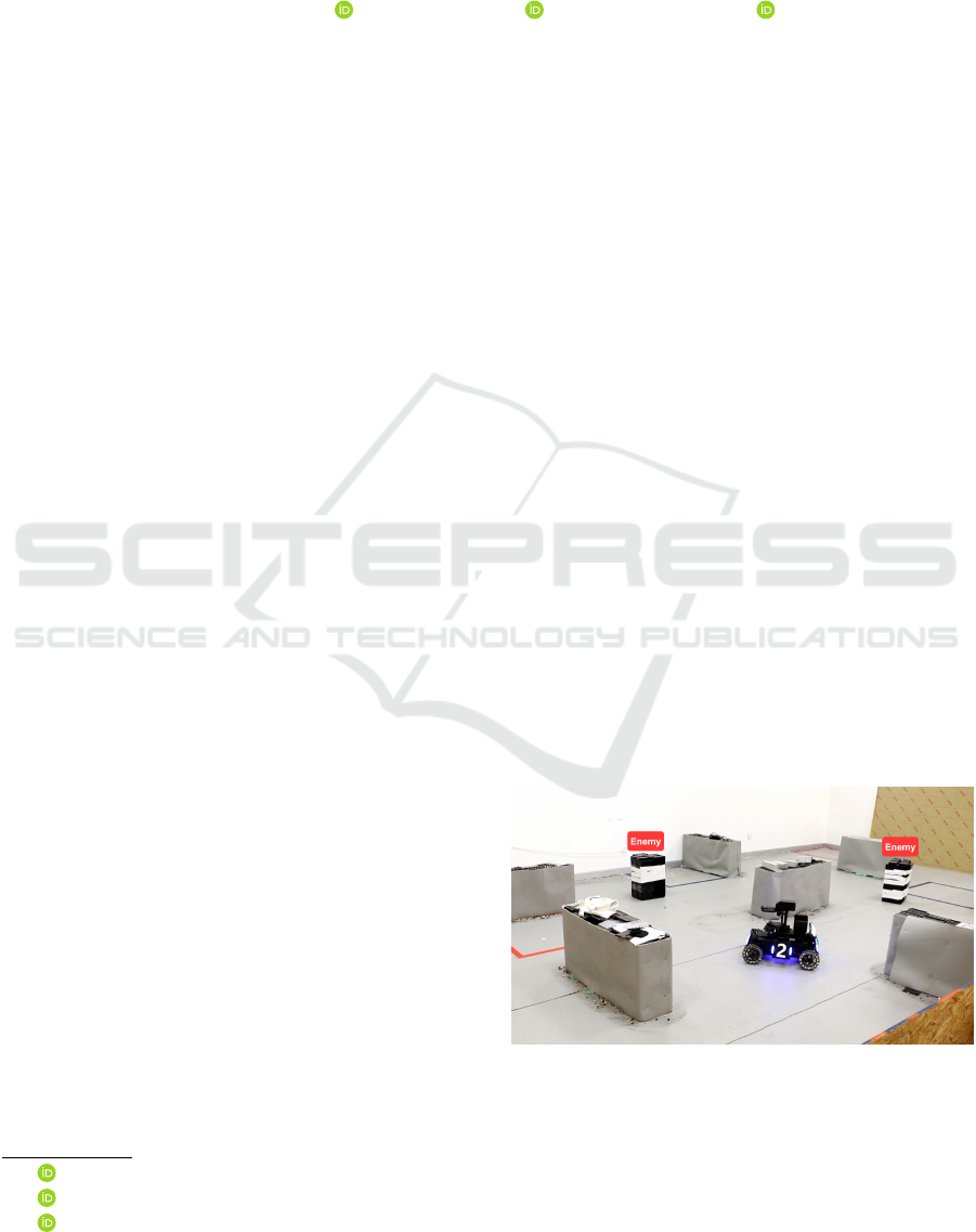
Figure 1: The arena used for experiments. As enemies don’t
change position during iterations, we use two plastic boxes
(in black, at the figure) to emulate their positioning, forcing
our robots to use LiDAR sensors to localize them.
Utill now, Deep PILCO has been applied on a
number of robotic tasks. (Gamboa Higuera et al.,
2018) improved Deep PILCO by using random num-
Huang, J., Giardina, F. and Rosendo, A.
Deep vs. Deep Bayesian: Faster Reinforcement Learning on a Multi-robot Competitive Experiment.
DOI: 10.5220/0010601905010506
In Proceedings of the 18th International Conference on Informatics in Control, Automation and Robotics (ICINCO 2021), pages 501-506
ISBN: 978-989-758-522-7
Copyright
c
 2021 by SCITEPRESS – Science and Technology Publications, Lda. All rights reserved
501

bers and clips gradients, and applied it for learning
swimming controllers for a simulated 6 legged au-
tonomous underwater vehicle. In (Kahn et al., 2017),
the authors learned the specific task of a quadrotor
and an RC car navigating an a priori unknown envi-
ronment while avoiding collisions using Deep PILCO
with bootstrap (Efron, 1982). The advantages of Deep
PILCO in learning speed have been proven on simu-
lations and single-robot experiments.
Here we propose, for the first time in the real-
world, applications of Deep Learning and Deep
Bayesian Learning on a multi-robot confrontation
game. Our experiments aimed to solve the decision
making problem of robots at the international IEEE
ICRA AI Challenge, a problem which was tackled
with a different approach in our previous work (Zhang
and Rosendo, 2019). We compare a Deep PILCO im-
plementation to a Deep Q Learning algorithm on this
very same experiment. Our results prove that Deep
PILCO significantly outperformed DQL in learning
efficiency and scalability, and these results are dis-
cussed in Section 4. We conclude pointing to the ad-
vantages of Deep Bayesian Reinforcement Learning
implementations over Deep Reinforcement Learning
when implemented in the real world.
2 PROBLEM DEFINITION
The real-world experiments were run using a robot
manufactured by DJI (Fig. 2). The robot’s different
hardware compositions sensed the environment and
provided sensory data for the experiment. LiDAR and
IMU collected data for the robot to localize both itself
and the enemy robots in the map. The camera helped
detect the armors of the enemy robots, which is essen-
tial to accomplish auto firing. Rasberry Pi and TX2
are two computing units of the robot.
RPLIDAR A3
CAMERA
RPLIDAR S1
NVIDIA TX2
IMU!
Figure 2: Hardware of the adopted robot. The robot is ca-
pable of recognizing the enemy through a combination of a
LiDAR and a camera, both sensors sampled by a TX2 and
a Raspberry Pi.
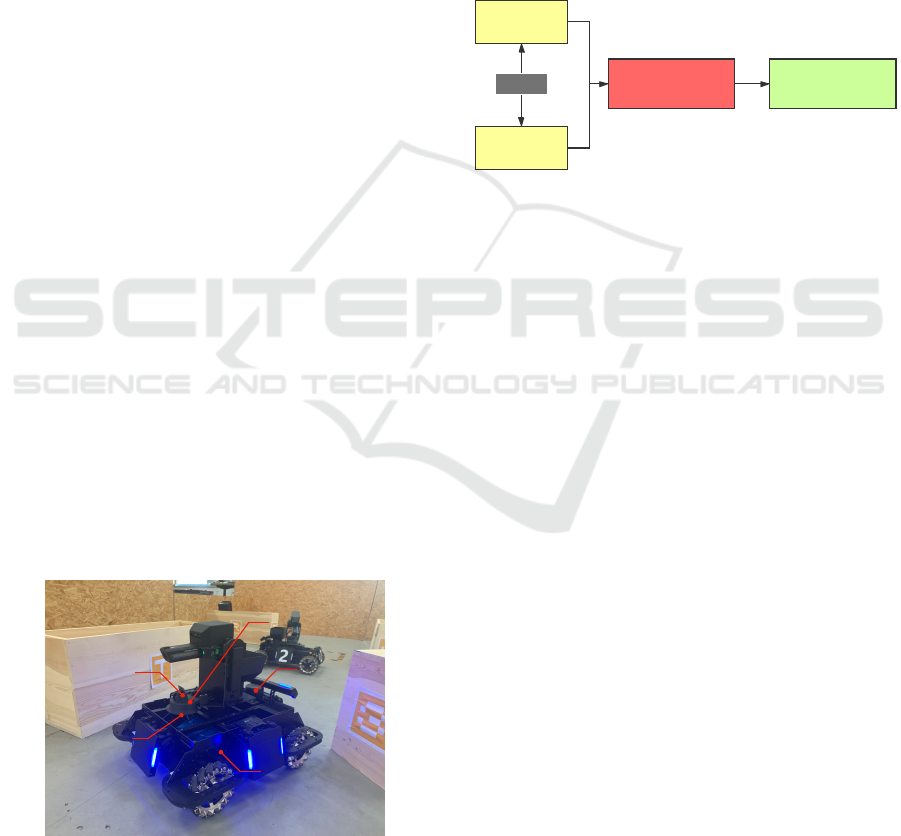
The multi-robot competitive problem was divided
into several sub-modules as shown in Fig. 3. LiDAR-
based localization module and enemy detection mod-
ule transferred the Cartesian coordinates of the robots
to decision making module as inputs. For decision
making module, we ran RL algorithms to obtain a pol-
icy search strategy. The strategy then generated a goal
position for the robot based on the current circum-
stance and sent it to the path planning module. After-
wards, path planning module planned a feasible path
on the map to let the robot arrive at the goal position.
In this paper, we focus on the implementation details
of the RL methods for the decision making module.
Decision Making Path Planning
Localization
Enemy
Detection
Lidar
Figure 3: Main modules of the multi-robot competitive
problem. We use Deep PILCO and DQL algorithms to train
a policy search strategy for the decision making module.
To fulfill the Markovian property requirement of
RL problems, we re-formulated the multi-robot com-
petitive problem to be a Markov Decision Process
(MDP) as follows. The MDP is composed of states,
actions, transitions, rewards and policy, which can be
represented by a tuple < S , A, T, R, π >.
• State: S is the state space which contains all pos-
sible states. Considering the map of the arena
is omniscient and path planning module is inde-
pendent to the RL algorithm, we projected the 3-
dimensional coordinate of the robot (x, y, z) to a
1-dimensional coordinate (p), where p represents
the position on the map. As shown in Fig. 4, the
original map was divided into 30 strategic areas
in advance. The size of each area depended on
the appearing possibility of the robot during the
match. Following this treatment, the state can be
denoted by a tuple (p
M
, p
E
n
, N
E
, p
M
) represents
the position of the robot itself. p
E
n
represents the
positions of the enemy robots, where n ∈ {1, 2} is
the index of the enemy robots. N
E
represents the
number of detected enemy robots discovered by
the LiDAR-based enemy detection function.
• Action: A is the action space which consists of
the actions the robot can take. For our problem,
an action (p
G
) is the next goal position for the
robot.
• Transition: T (s
0
|s, a) is the transition distribution
ICINCO 2021 - 18th International Conference on Informatics in Control, Automation and Robotics
502

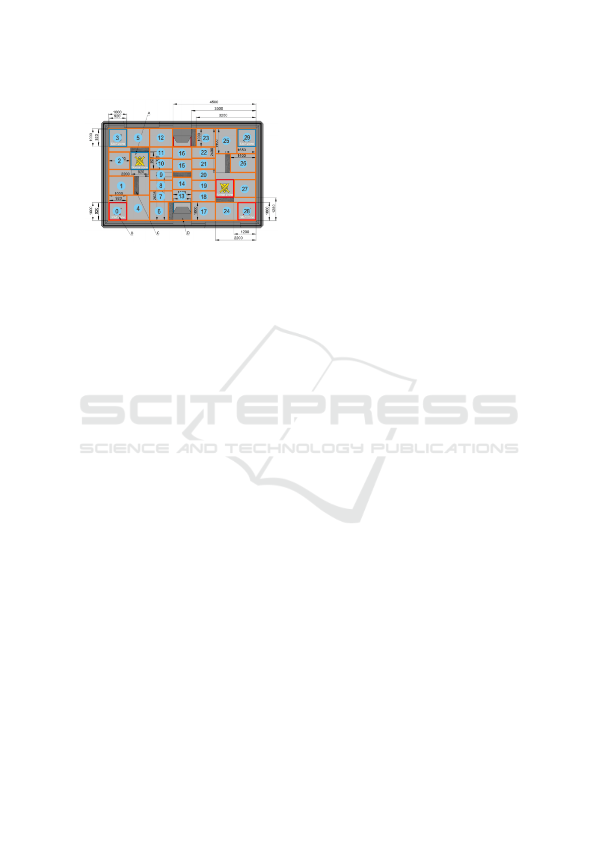
Figure 4: The original arena on the top is divided into 30
strategic areas to discretize the state space, as shown in the
figure below. In the original map, the red and blue squares
indicate the special regions in the competition, such as start-
ing zones and bonus zones. These marks can be ignored in
our experiments.
over the next state s
0
, given the robot took the ac-
tion a at the state s.
• Reward: R(s) is the immediate reward function
over state s. For this experiment, the reward was
computed merely based on the number of visible
enemy robots of the state s.
R(s) =

0, s[N
E
] 6= n (1a)
1, s[N
E
] = n (1b)
where n is the target number of visible enemy
robots.
• Policy: π(a|s) is a probability distribution of all
actions under the state s. The action to be taken is
given by the policy based on the state.
3 MATERIALS AND METHODS
3.1 Experimental Design
We ran the experiments in two cases. The first case
was 1v1 design, which meant there was only one
robot against one enemy robot, while the second case
was 1v2 design, as there were one robot against two
enemy robots.
The enemy robots kept static at one place during
each episode. Therefore, we could just use boxes of
similar sizes with the robot to represent enemy robots,
as shown in Fig. 1.
3.2 Experimental Methods
3.2.1 Deep Q-Learning
Q-Learning (Watkins and Dayan, 1992) algorithms
aim to solve an MDP by learning the Q value func-
tion Q(s, a). Q(s, a) is a state-action value function,
which gives the expected future return starting from a
particular state-action tuple. The basic idea is to esti-
mate the optimal Q value function Q
∗
(s, a) by using
the Bellman equation as an update:
Q
∗
(s, a) = E
s
0
[r + γ max
a
0
Q
∗
(s
0
, a
0
)|s, a]. (2)
DQL is a variant of the Q-Learning algorithm, which
takes a deep neural network as a function approxima-
tor for the Q value function where samples are gen-
erated from the experience replay buffer. Note that
DQL is model-free: it solves the RL task directly
using samples from the emulator, without explicitly
constructing an estimate of the emulator (or transition
model) (Mnih et al., 2016). Instead of updating the
policy once after an episode in the model-based al-
gorithm PILCO (Deisenroth and Rasmussen, 2011),
DQL updates the Q-network with samples from the
replay buffer every step.
We implemented the DQL algorithm using the
Tianshou library (Weng et al., 2020), whose underly-
ing layer calls the pytorch library (Paszke et al., 2019)
for neural network-related computations. As for the
model architecture, the input to the Q-network is a
state vector. The two hidden layers consist of 128
neurons for simulations, 16 neurons for experiments,
activated by ReLU function (Nair and Hinton, 2010).
The output layer is a fully-connected linear layer with
a single action output. The policy during training is ε-
greedy at ε = 0.1. The learning rate is 0.001, and the
discount factor is 0.9. The size of the replay buffer is
20000.
3.2.2 Deep PILCO
Compared to model-free deep RL algorithms, model-
based RL allows higher sample efficiency, which can
be further improved with a probabilistic transition
model. Deep PILCO is a prominent example which
utilizes a Bayesian neural network (BNN) (MacKay,
1992) to estimate the transition model (Gal et al.,
2016; Gamboa Higuera et al., 2018).
The algorithm can be summarized as follows: A
policy π’s functional form is chosen from scratch,
with randomly chosen parameters φ. Then, Deep
PILCO executes the current policy on the real agents
from the current state until the time horizon T . The
new observations are recorded and appended to the
Deep vs. Deep Bayesian: Faster Reinforcement Learning on a Multi-robot Competitive Experiment
503

whole dataset, from which a new probabilistic tran-
sition model (or more precisely, the model parame-
ters of BNN) is re-trained. Based on this probabilistic
transition model, Deep PILCO predicts state distribu-
tions from the current initial state distribution p(X
0
)
to p(X
T
). In detail, the state input and output uncer-
tainty are encoded by using particle methods. Pro-
vided with the multi-state distribution p(X
0
, ..., X
T
),
the cumulative expected cost J(φ) is computed, with
a user-defined cost function. By minimizing this ob-
jective function (using gradient descent method), a
newly optimized policy π
φ
is obtained. Note that here
we defined the cost function opposite to the reward:
Cost(X ) = 1 − R(X).
We implement Deep PILCO in an episodic way
so that the algorithm updates the policy after every
episode based on the episodic rewards. The episodic
reward is the sum of iteration rewards. Each episode
consists of 10 iterations. During one iteration, the
robot moves from the current position to the goal
position given by the action along the planned path.
The code is a modified version of an open-source
implementation of Deep PILCO algorithm (Gam-
boa Higuera et al., 2018).
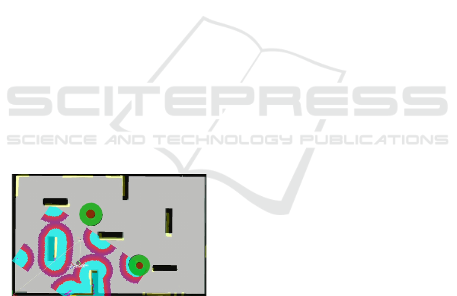
3.2.3 LiDAR-based Enemy Detection Function
We used a 2d obstacle detection algorithm to extract
obstacles information from lidar data. Since we knew
the map, we knew where the walls are. If the center
of a robot was inside a wall, we filtered out this cir-
cle (Zhang and Rosendo, 2019). A screenshot taken
during the algorithm running is presented in Figure 5.
Figure 5: The visualization of the LiDAR-based enemy de-
tection algorithm. The position of the plastic boxes (ene-
mies) are shown in the two green circles. The navigation
stack in ROS depicts the contour of the obstacles in yellow,
and displays the local costmap in blue, red and purple.
4 RESULTS
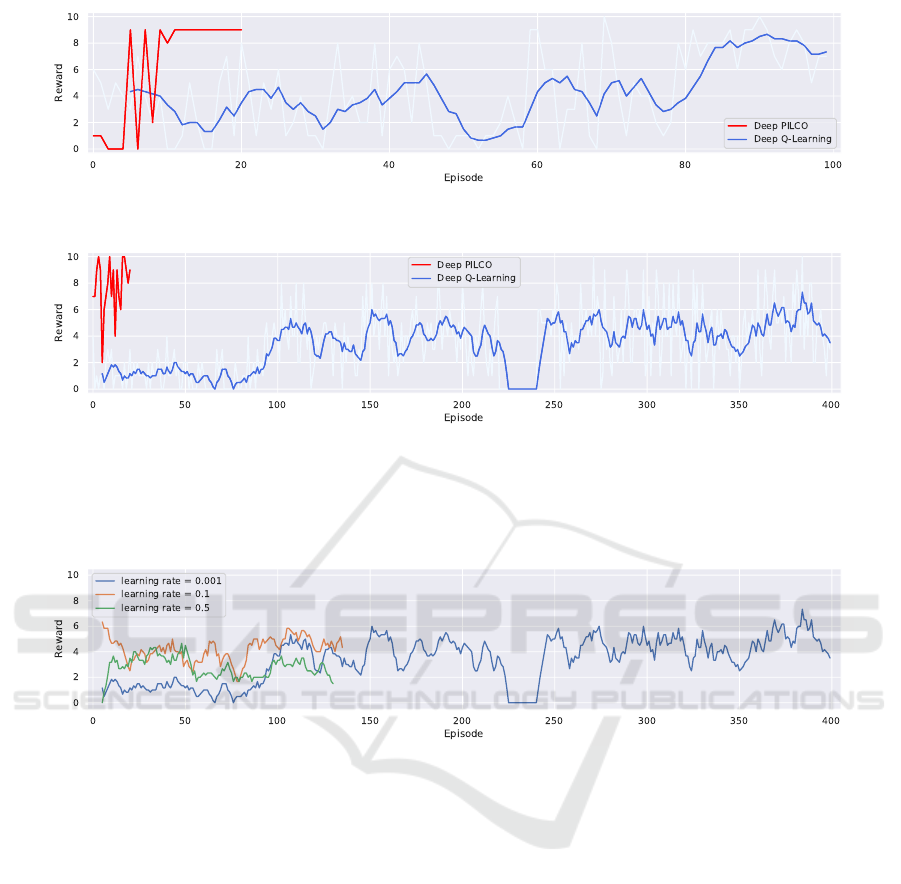
We first compare the episodic rewards of DQL and
Deep PILCO. In order to reveal the learning trend,
we also plot the rolling mean rewards of six neigh-
boring episodes for DQL. For the 1v1 case, both al-
gorithms learned optimal solutions after training. In
Fig. 6(a), we can see that Deep PILCO found the
solution within 11 episodes, much fewer than DQL,
which took around 90 episodes. Furthermore, the re-
sult of Deep PILCO stayed maximal after the optimal
moment, while the result of DQL was more unsteady.
For the 1v2 case, the results of both algorithms
fluctuated more than in the 1v1 case, as shown in Fig.
6(b). While the performance of Deep PILCO kept a
similar number of episodes when changing from the
1v1 case to the 1v2 case, DQL failed to converge to
an optimal solution even after 400 training episodes.
Considering the expensive training cost of real-
world experiments, we stopped the experiment after
400 episodes. To eliminate the impact of the hyper
parameters, we changed the learning rate parameter of
DQL algorithm and reran the experiments, but DQL
was still unable to find a stable optimal solution, as
we can see in Fig. 7.
With regards to computation time, fewer train-
ing episodes are not necessarily equivalent to shorter
training time, since each episode costs different clock
time for DQL and Deep PILCO. For both algorithms,
each episode contains 10 iterations, while each itera-
tion costs about 10 seconds to run. With regards to the
computation time, Deep PILCO takes approximately
1 minute per episode, while DQN takes 3 seconds
per episode. To sum up, the training time for Deep
PILCO is 160 seconds per episode, and 103 seconds
per episode for DQL.
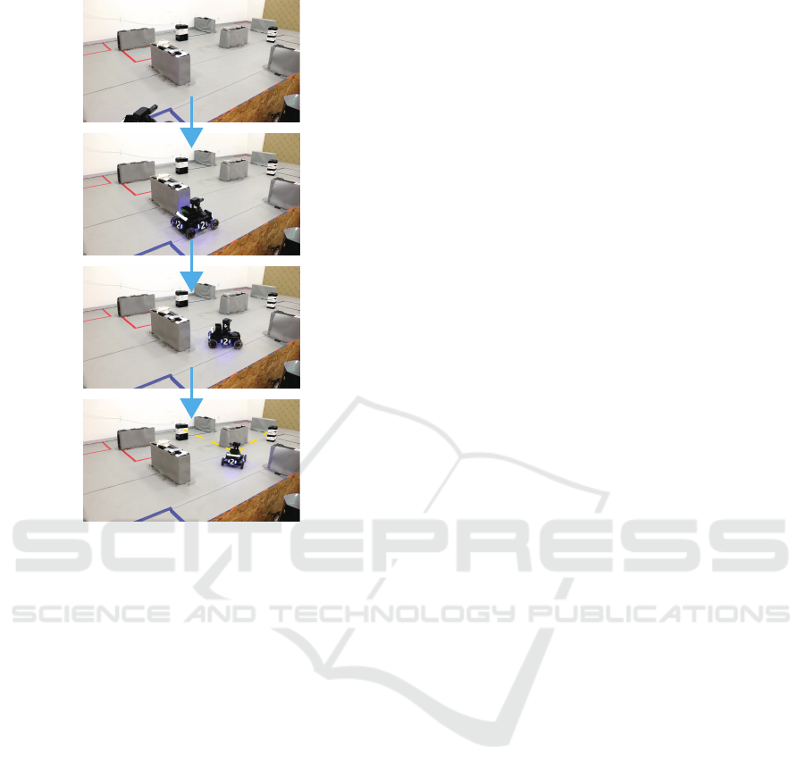
Fig. 8 displays the snapshots of our experiments
with Deep PILCO for 1v2 case. The four pictures
show different phases of the found optimal policy. We
can see that our robot started from the initial state,
where it saw none of the enemy robots, and finally
navigated to an optimal position where it could see
two enemy robots at the same time. In the rest of the
episode, it stayed at the optimal position in order to
achieve a highest episodic reward.
5 DISCUSSION
Experimental results show that Deep Bayesian RL
surpassed Deep RL in both learning efficiency and
learning speed. This confirms the findings of previ-
ous works in (Deisenroth and Rasmussen, 2011; Gal
et al., 2016). Although for each iteration, the calcula-
ICINCO 2021 - 18th International Conference on Informatics in Control, Automation and Robotics
504

(a) 1v1 case
(b) 1v2 case
Figure 6: Learning curves tracking the rewards over episodes. Deep PILCO and Deep Q-Learning were running with learning
rate α = 0.001. (a) Training rewards of DQL and Deep PILCO for 1v1 case. The red curve vanished earlier since Deep
PILCO converged to the optimal reward within fewer training episodes. (b) Training rewards of DQL and Deep PILCO for
1v2 case.
Figure 7: Training results of 3 different learning rate setup for Deep Q-Learning in 1v2 case. Empirically, learning rates with
large values hinder the convergence in DQL experiments. With that in mind we ran more trials with the smallest learning rate
0.001. Nonetheless, all three experiments fail to achieve a reasonably high reward.
tion time requires for DQL is much shorter than that
of Deep PILCO, the learning efficiency of the latter
makes up for the cost. The transistors on a chip will
double in each generation of technology as claimed
by Moore’s law. We presume that Deep Bayesian
RL algorithms will learn policies much faster than
Deep RL, with foreseeable more advanced computa-
tion hardware.
The first few training episodes of Deep PILCO in
1v2 case achieved higher initial reward than 1v1 case,
as we can see in Figure 6. This is the result of a better
exploration of the initial random rollouts in the 1v2
case. Yet in our experiments, the larger number of
initial random rollouts did not guarantee the higher re-
wards, which verifies the finding in (Nagabandi et al.,
2018). In this work, they evaluated various design de-
cisions in model-based RL algorithms, including the
number of initial random trajectories. They found that
low-data initialization runs were able to reach a high
final performance level as well, due to the reinforce-
ment data aggregation.
6 CONCLUSIONS
We proposed a new application of Deep PILCO on
a real-world multi-robot combat game. We further
compared this Deep Bayesian RL algorithm with
the Deep Learning-based RL algorithm, DQL. Our
results showed that Deep PILCO significantly out-
performs Deep Q-Learning in learning speed and
scalability. We conclude that sample-efficient Deep
Bayesian learning algorithms have great prospects on
competitive games where the agent aims to win the
opponents in the real world, as opposed to being lim-
ited to simulated applications.
Deep vs. Deep Bayesian: Faster Reinforcement Learning on a Multi-robot Competitive Experiment
505

Initial state
Figure 8: Snapshots of the real-world experiment for the 1
vs 2 situation. After about 15 training episodes, the robot
found the optimal position to see the two enemies simulta-
neously. During the episode that the reward is the highest,
the robot started from the initial position, and then navi-
gated to the optimal place at the end of the first iteration.
The robot stayed at the optimal place during the rest of the
episode to get a maximal reward.
REFERENCES
Chua, Kurtland and Calandra, Roberto and McAllister,
Rowan and Levine, S. (2018). Deep Reinforcement
Learning in a Handful of Trials using Probabilistic
Dynamics Models. Advances in Neural Information
Processing Systems, (NeurIPS):4754—-4765.
Deisenroth, M. P. and Rasmussen, C. E. (2011). PILCO:
A model-based and data-efficient approach to policy
search. Proceedings of the 28th International Confer-
ence on Machine Learning, ICML 2011, pages 465–
472.
Depeweg, S., Hernández-Lobato, J. M., Doshi-Velez, F.,
and Udluft, S. (2019). Learning and policy search
in stochastic dynamical systems with Bayesian neural
networks. 5th International Conference on Learning
Representations, ICLR 2017 - Conference Track Pro-
ceedings, pages 1–14.
Efron, B. (1982). The jackknife, the bootstrap, and other
resampling plans, volume 38. Siam.
Gal, Y., Mcallister, R. T., and Rasmussen, C. E. (2016). Im-
proving PILCO with Bayesian Neural Network Dy-
namics Models. Data-Efficient Machine Learning
Workshop, ICML, pages 1–7.
Gamboa Higuera, J. C., Meger, D., and Dudek, G. (2018).
Synthesizing Neural Network Controllers with Proba-
bilistic Model-Based Reinforcement Learning. IEEE
International Conference on Intelligent Robots and
Systems, pages 2538–2544.
Gu, S., Lillicrap, T., Sutskever, U., and Levine, S. (2016).
Continuous deep q-learning with model-based accel-
eration. 33rd International Conference on Machine
Learning, ICML 2016, 6:4135–4148.
Kahn, G., Villaflor, A., Pong, V., Abbeel, P., and
Levine, S. (2017). Uncertainty-aware reinforcement
learning for collision avoidance. arXiv preprint
arXiv:1702.01182.
Lillicrap, T. P., Hunt, J. J., Pritzel, A., Heess, N., Erez, T.,
Tassa, Y., Silver, D., and Wierstra, D. (2016). Contin-
uous control with deep reinforcement learning. 4th In-
ternational Conference on Learning Representations,
ICLR 2016 - Conference Track Proceedings.
MacKay, D. J. (1992). Bayesian Methods for Adaptive
Models. PhD thesis, California Institute of Technol-
ogy.
Mnih, V., Kavukcuoglu, K., Silver, D., Graves, A.,
Antonoglou, I., Wierstra, D., and Riedmiller, M.
(2016). Playing Atari with Deep Reinforcement
Learning.
Nagabandi, A., Kahn, G., Fearing, R. S., and Levine, S.
(2018). Neural Network Dynamics for Model-Based
Deep Reinforcement Learning with Model-Free Fine-
Tuning. Proceedings - IEEE International Conference
on Robotics and Automation, pages 7579–7586.
Nair, V. and Hinton, G. E. (2010). Rectified linear units
improve restricted boltzmann machines. In Icml.
Paszke, A., Gross, S., Massa, F., Lerer, A., Bradbury, J.,
Chanan, G., Killeen, T., Lin, Z., Gimelshein, N.,
Antiga, L., et al. (2019). Pytorch: An imperative
style, high-performance deep learning library. arXiv
preprint arXiv:1912.01703.
Rusu, A. A., Vecerik, M., Rothörl, T., Heess, N., Pascanu,
R., and Hadsell, R. (2017). Sim-to-Real Robot Learn-
ing from Pixels with Progressive Nets. 1st Conference
on Robot Learning, CoRL 2017, (CoRL):1–9.
Watkins, C. J. and Dayan, P. (1992). Q-learning. Machine
learning, 8(3-4):279–292.
Weng, J., Zhang, M., Duburcq, A., You, K., Yan, D., Su,
H., and Zhu, J. (2020). Tianshou. https://github.com/
thu-ml/tianshou.
Zhang, Y. and Rosendo, A. (2019). Tactical reward shaping:
Bypassing reinforcement learning with strategy-based
goals. IEEE International Conference on Robotics
and Biomimetics, ROBIO 2019, (December):1418–
1423.
ICINCO 2021 - 18th International Conference on Informatics in Control, Automation and Robotics
506