Towards Automatic Detection and Quantification of Mildew on

Grape Leaf Disks

Razib Iqbal, Kyle Sargent and Laszlo Kovacs

College of Natural and Applied Sciences, Missouri State University, Springfield, MO, U.S.A.

Keywords: Background Removal, Downy Mildew, Grape Leaf, HSV Masking, Image Analysis.

Abstract: Downy and powdery mildews are the most serious diseases of the grapevine. A sustainable way to control

these pathogens is the breeding and deployment of resistant grape cultivars. For breeding efforts to be

effective, accurate quantification of the resistance phenotype is essential. In this paper, we present a computer-

based image recognition, processing, and analysis technique for enhancing the detection and quantification of

Plasmopara viticola and Erysiphe necator the causal agents of downy and powdery mildew, respectively. We

propose a multi-step approach that utilizes background removal and Hue-Saturation-Value (HSV) masking

as opposed to multi-faceted color channel breakdowns, photo texture evaluations, or classification-based

algorithms for the detection of mildew. Our experimental results show that our method provides reliable

results and fast performance.

1 INTRODUCTION

Plants can be classified based on two distinctions of

infection, namely, non-infected (or normal) and

infected (Awate et al, 2015). In the infected plants

category, the growth of pathogen on plants is a major

problem in the agricultural industry. To prevent it,

many cultivators turn to harmful pesticides to

slow/prevent the infection of it. While this practice is

effective, it has many drawbacks. Instead, biologists

have looked into breeding the plants selectively in

order to breed samples that are naturally resistant to

certain pathogens. In order to determine success in

this manner, we need to analyze infected samples and

determine the rate and amount of growth of infection

on those samples. In this paper, we focus on grape leaf

disks and the methods for detection and quantification

of the mildew at both the microscopic level and

human eye-level.

The existing methods for detecting mildew

include color-space analysis, texture analysis, support

vectors, and visual analysis (Awate et al, 2015;

Sandika et al, 2016; Li et al, 2011; Vijayakumar,

2012). Hardware-based image analyses, such as

(Cruz et al, 2016), rely on the capabilities of the

hardware and the cost of the hardware is a factor in

determining the aspects of the analysis. In

comparison, visual analysis even though the most

accessible and cost-efficient detection method has

factors of bias from human perception. Its primary

use is when quick and non-accurate readings are

required to give a baseline for further analysis at a

later point. Since this method is often accompanied

by result variation, we have turned to computer-based

image analysis for reliable and deterministic output

that is useful to the end user.

Color space analysis can be further divided into

multiple different categories, such as RGB color-

space analysis, BGR color-space analysis and Hue-

Saturation-Value (HSV) color space analysis. As per

(Vijayakumar, 2012), the RGB color-space can be

split between the individual color channels to point

out anomaly values caused by the growth of mildew.

This method allows for a histogram approach, which

accompanies calculating the mean value of each color

channel and tracking changes in said values. HSV and

BGR color spaces, also maintain the abilities from the

RGB color-space analysis technique. However,

creating a histogram of all colors in a single image

can be very cumbersome on a machine depending on

two factors: image quality and image resolution. Due

to this, we elected to use color space masking to

alleviate the necessity of histogram creation or any

other expensive color channel tracking approaches.

Our proposed approach tends to provide a reliable

method for quantifying the mildew growth on grape

leaves.

Iqbal, R., Sargent, K. and Kovacs, L.

Towards Automatic Detection and Quantiﬁcation of Mildew on Grape Leaf Disks.

DOI: 10.5220/0010583900810086

In Proceedings of the 18th International Conference on Signal Processing and Multimedia Applications (SIGMAP 2021), pages 81-86

ISBN: 978-989-758-525-8

The rest of the paper is organized as follows: In

Section 2, we present our proposed approach with the

implementation details. In Section 3, we present our

performance evaluation. Finally, in Section 4, we

conclude this paper with our observation followed by

our future plans.

2 PROPOSED APPROACH

In order to measure the rate of mildew on the disk leaf

samples we apply Background Removal (BR) and

HSV masking to eliminate non-mildew spots from

each photo samples. We then use the Laplacian of

Gaussian (LoG) blob detection algorithm to quantify

the amount of mildew contained in each photo. We

explain these steps in the following subsections.

2.1 Image Acquisition

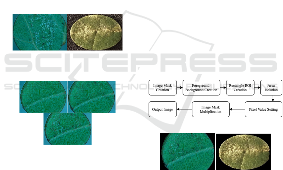
Figure 1: Photos of leaf disks infected with downy-and

powdery-mildew at the micro- (left) and macroscopic-level

(right).

Figure 2: Single downy mildew-inoculated leaf disk over

six-day span (left, right, bottom: 2dpi, 4dpi, 6dpi).

For our research, grape plants are cultivated as normal

and given time to grow into mature vines. Once the

plant has reached this stage, circular disks are cut

from the plant’s leaves, thus, supplying a grape leaf

disk. These disks are then inoculated with P. viticola

or E. necator as shown in Figure 1, and tracked over

a six-day period. Throughout these six days, the

growth of the mildew is tracked and photographs of

the leaf disks at the macroscopic level are taken in the

lab setting. On the sixth day, the resistance to the

mildew is determined based on the extent of growth,

which inversely related to disease resistance. During

this process, visual analysis is conducted to deduce a

baseline approximation of mildew on the leaf disk

and resistance to the mildew.

The downy mildew images we used for this research

were acquired from the laboratory of Dr. Lance

Cadle-Davidson at the USDA Agricultural Research

Service (Bierman et al, 2019). Our database included

53 photos in total with 48 of them being at the

microscopic level and 5 being at the human eye level.

The 43 microscopic photos span from 2-, 4-, and 6-

days past inoculation (dpi) of the leaf disk with the

mildew and photos were taken under lab-grade

microscopes and photo equipment with generally

consistent lighting placement of leaf disks within the

photos as shown in Figure 2. The macroscopic photos

of powdery mildew infected leaf disks were taken

with a USB camera with varying days past

inoculation and varying distances from the disk under

consistent lighting condition.

2.2 Background Removal

Background removal is the method in which the

isolation of the leaf disk in the photo is done. This

step is necessary because if the background has a

similar color to that of the mildew, then false positive

readings for mildew can occur. The steps for

background removal are shown in Figure 3 and the

respective outputs are shown in Figure 4.

Figure 3: Steps for background removal.

Figure 4: Background removed mirco- and macro- scopic

level photos.

2.3 HSV Masking

HSV masking is the phase where the areas within the

leaf disk that do not contain what is classified as

mildew are masked out prior to blob detection and

quantification. To accomplish this, an image’s color-

space must be converted from BGR to HSV. The set

of equations in (1) and (2) are used to convert 8/16-

bit images from BGR color space to HSV color space.

SIGMAP 2021 - 18th International Conference on Signal Processing and Multimedia Applications

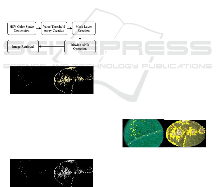
Since BGR values can only lie between 0 and 255,

and HSV values lie between 0 and 255 for both

Saturation and Value and 0-360 for Hue, an extra step

of conversion is necessary to fit the Hue values

between 0 and 255 for 8-bit images.

V → max(R,G,B)

S → { V – min(R,G,B) if V ≠ 0

0 otherwise }

H → { 60(G-B)/(V – min(R,G,B)) if V = R

120 + 60(B-R)/ (V-min(R,G,B)) if V = G

240 + 60(R-G)/(V-min(R,G,B)) if V = B }

(1)

H → H /2

(2)

Since HSV is in three-dimensional space, two

threshold arrays or vectors are created to specify a

minimum and maximum threshold value. With this

threshold, utilizing the third number, namely the

value we want to mask over, allows us to keep only

pixels whose value surpasses that of the minimum

threshold. The steps to complete HSV masking are

shown in Figure 5 and the respective output is

presented in Figure 6.

Figure 5: HSV masking steps.

Figure 6: Output from HSV masking on micro- and

macroscopic-level photos respectively.

2.4 Blob Detection

Blob detection is where the quantification of the

mildew occurs. Once the masking has been

completed, the resulting image that contains what is

assumed to be mildew is once again converted to

grayscale. The grayscale images shown in Figure 7

are computed by equation (3).

Figure 7: Grayscale version of sample photos after HSV

masking.

Y → 0.299 · R + 0.587 · G + 0.114 · B

(3)

g(x,y,t) = (1/2πt) · e

-(x²+y²)/2t

(4)

L(x,y;t) = g(x,y,t) ꞏ f(x,y)

(5)

Once the grayscale image is returned, we then

utilize Blob detection for quantification of the

mildew. There are three types of Blob detection

algorithms that we initially considered - Laplacian of

Gaussian, Difference of Gaussians and Determinant

of Hessian. We chose to use the Laplacian of

Gaussian approach since it gave us the most accurate

and fastest output of the three. We capture the

different size blobs found throughout the image using

the equations in (4)-(7).

Equation (4) is used to convolve the input image,

which produces a third equation that dictates how one

function is shaped by another. Equation (5) shows the

scale space representation of the original image after

the convolution. The scale space representation is

essentially a representation of the photo, with a

Gaussian filter on it that amplifies as the scale t grows

in number. Then we apply the Laplacian Operator (6)

to (5) that determines the blobs of scale t as per

(Lindeberg, 2013).

▲²L = L

+ L

(6)

Following the application of (6) to (5), the

Laplacian of Gaussian algorithm outputs the

following:

detectedBlob = (x, y, σ)

(7)

Here, (x, y) are the coordinates of the blob and σ

is the standard deviation of the gaussian kernel which

detected the blob. Now, the radius of a single blob is

≈ √2 σ. At this point, we use equation (8) to obtain the

radius of the blob.

r = σ · √2

(8)

A = π · r²

(9)

Figure 8: Detected blobs on micro- and macroscopic-level

photos.

Now that we have the radius of said blob at

coordinates (x,y), we find the area of a circle with said

radius found by using (9). We can draw circles for n

blobs that were detected in the photo, as shown in

Figure 8, and sum their areas together to retrieve the

total area taken up by the blobs on a single leaf disk

Towards Automatic Detection and Quantiﬁcation of Mildew on Grape Leaf Disks

in pixel units. Once we retrieve all of the blob areas,

we then use equation (11) to compute a leaf to mildew

ratio.

TotalBlobArea = Σ A

(for i =0 to i=n)

(10)

TotalBlobArea/NonBlackPixelsAfterBR · 100

(11)

3 EVALUATION

Table 1: Mildew growth over a 6-day period.

Tray

Number

Photo

Number

Mildew %

at 2dpi

Mildew % at

4dpi

Mildew %

at 6dpi

1 1 0.1193466 0.0 0.0055978

2 1 0.9503586 0.0413495 0.0117653

3 1 0.0061946 0.33576335 0.0369914

4 1 0.3733049 0.3357633 0.3462468

5 1 0.1799363 0.097927 0.1035048

6 1 0.3605445 0.4817453 0.0835825

7 1 0.0625684 0.0995543 0.092579

8 1 0.0550063 0.0791701 0.175554

1 2 1.6531951 1.3868999 2.173476

2 2 0.5955877 0.5151023 0.3470667

We tested our approach in two facets: growth tracking

and quantification/detection. The growth tracking

ability of our approach was tested by selecting a

singular plant and tracking its mildew growth. This

test was conducted on 10 of the 48 microscopic level

images. For the data presented in Table I, we tested

10 different samples over a six-day span. From the

reported results, we observed two trends, namely,

decreasing and increasing. However, the other trend

shown in the table, by rows 1 and 9, is that of

fluctuation. This trend is caused by the thresholding

aspect of the approach and the appearance of cell

structures that closely resemble the coloring of the

mildew. Also, the mildew requires viable cells to live

in, and therefore, if cells die then so does the mildew.

This phenomenon causes fluctuation in the amount of

mildew detected and quantified over the test period.

For quantification/detection evaluation, we tested

on two different computers - a laptop with 8GB of

RAM with an Intel Core i7 CPU @ 2.80GHZ

processor and a desktop with 32GB of RAM with an

Intel Core i7 CPU @ 3.2GHz processor. We will refer

to these two test machines as Machine A and Machine

B, respectively.

Table 2: Leaf to mildew ratios - Machine A.

Days Past

Inoculation

(DPI)

Photo Date

Tray

Number

Photo

Number

Mildew %

(pixels)

2 9-15-18 3 1 0.0

6 9-19-18 5 2 0.1533935

6 9-19-18 7 2 1.4873933

6 9-19-18 1 1 0.0059786

6 9-19-18 8 1 0.1755536

6 9-19-18 6 1 0.0835783

4 9-17-18 4 1 0.3357634

4 9-17-18 2 1 0.0413495

2 9-15-18 1 2 1.6531951

2 9-15-18 3 2 0.8965174

Table 3: Leaf to mildew ratios - Machine B.

Days Past

Inoculation

(DPI)

Photo Date

Tray

Number

Photo

Number

Mildew %

(pixels)

4 9-17-18 2 2 0.0059078

2 9-15-18 4 1 0.07149801

2 9-15-18 5 1 0.05584116

6 9-19-18 1 1 0.0

6 9-19-18 7 1 0.0555477

6 9-19-18 8 1 0.1271250

4 9-17-18 3 1 0.0651918

4 9-17-18 6 1 0.2470763

2 9-15-18 6 2 0.0609538

2 9-15-18 8 2 0.4067885

We tested the system with the following tests: 1

photo, 2 photos, 3 photos, 4 photos, up to 8 photos at

a time. Since we tested a total of 36 photos per test for

Tables II and III, we display only the first 10 results

without losing any important information. In Table II,

we showcase the quantification results from Machine

A, and in Table III, we showcase the results from

Machine B. Photos were chosen at random from three

date folders of 9-15-18, 9-17-18 and 9-19-18 and then

from one of the 8 tray folders within each date. The

photos selected for this test were also solely at the

microscopic level since the macroscopic-level photos

SIGMAP 2021 - 18th International Conference on Signal Processing and Multimedia Applications

did not belong to a specific date folder. The mildew

percentages are in terms of pixel which is calculated

by dividing the number of pixels that existed after

removing the background by the number of pixels the

blobs of mildew took up. Higher density of mildew

produces a higher mildew percentage overall. Since

these numbers are computer generated, they were

same for both machines, which is why we chose the

photos at random for both machines. Also, for the two

machines, there was a difference in the HSV mask

threshold values. The 8GB machine ran with a

threshold value of 170 and the 32GB machine ran

with a threshold of 180. This explains the difference

in the outputs of row 4, column 5 in both Tables II

and III.

Table 4: Detection-Quantification runtimes - Machine A.

# of

Tested

Photos

Avg.

Detection

Runtime

(ms)

Total

Detection

Runtime

(ms)

Avg.

Quantification

Runtime (ms)

Total

Quantification

Runtime (ms)

1 1.3819 1.3819 374.1365 374.1365

2 5.85395 11.70789 498.7908 997.5817

3 129.16577 387.4973 649.2774 1947.83229

4 104.20022 416.80089 976.5763 3906.30529

5 14.38234 71.91169 823.5583 4117.79159

6 40.49657 249.7939 958.8845 5753.307709

7 53.75931 376.151 1031.3986 7219.79089

8 60.03296 480.2636 1451.8371 11614.6974

Table 5: Detection-Quantification runtimes - Machine B.

# of

Tested

Photos

Avg.

Detection

Runtime

(ms)

Total

Detection

Runtime

(ms)

Avg.

Quantification

Runtime (ms)

Total

Quantification

Runtime (ms)

8.4423 8.4423 274.828 274.828

4.9833 9.9665 371.36 742.721

79.1446 237.4338 349.585 1048.750

68.0872 272.3490 646.065 2584.260

66.904 334.5221 1062.229 5311.147

59.927 359.5607 1151.012 6906.069

13.547 94.8268 1050.920 7356.4422

76.119 608.9588 1416.313 11330.505

Table IV and Table V showcase the detection-

quantification run-time performance for 8 different

tests. As expected, we see a trend in which as the

numbers increase, the total and average times

increase as well. However, depending on the amount

of quantification or detection time that one photo

takes depend on the amount of mildew that resides

within the photo itself. Again, as with the mildew

percentages found in Tables II and III, less resistant

plants will take a longer time to detect and quantify

the mildew that resides on the leaf disks.

4 CONCLUSIONS

In this paper, we proposed a multi-step approach for

the detection and quantification of mildew diseases

that reside on either the top or the bottom of grape

leaves. We are working towards a fully automated

detection process to perform quantitative analysis of

the mildew growth in an outdoor setting. It will add

value to the process of selectively breeding grapes

based on their resistance.

The approach presented in this paper contains the

ability to detect and quantify mildew at both the

microscopic and macroscopic level. To acclimate to

the issue of thresholding, we used a number between

170 to 180 to retrieve the most optimal results. Any

value less than 170 for the set of photos we used

allowed for more cell structures and anomalies within

the photo, e.g., lens flare from the camera and

microscope, to be captured and identified as mildew

as well. Therefore, we recommend that a threshold

number between 170 and 180 be used to eliminate

majority of the false positives that could occur during

detection.

We also observed that the utilization of a blur

while thresholding allowed for more accurate results.

Because of the intricacies of the cells, the blue helped

to soften some of the cell pixels that could produce

false positives. To accomplish this, a gaussian blur of

3 was applied on the photos and anything higher

causes pixels to become too blurry for the blob

detection algorithm to pick them up correctly.

In the future, we plan to continue adjusting

threshold values and begin testing the approach with

more than just grape leaf disks to determine if the

approach can successfully capture mildew diseases of

other kinds that may grow on other plants as well. An

example could be, looking at the powdery mildew,

known as Podosphaera leucotricha, that grows on

apples.

Towards Automatic Detection and Quantiﬁcation of Mildew on Grape Leaf Disks

REFERENCES

Awate, A., Deshmankar, D., Amrutkar, G., Bagul, U., &

Sonavane, S. (2015). Fruit disease detection using

color, texture analysis and ANN. 2015 International

Conference on Green Computing and Internet of Things

(ICGCIoT), pp. 970-975.

Bierman, A., LaPlumm, T., Cadle-Davidson, L., Gadoury,

D., Martinez, D., Sapkota, S., & Rea, M. (2019). A

high-throughput phenotyping system using machine

vision to quantify severity of grapevine powdery

mildew. Plant Phenomics.

Cruz, J. A., Yin, X., Liu, X., Imran, S. M., Morris, D. D.,

Kramer, D. M., & Chen, J. (2016). Multi-modality

imagery database for plant phenotyping. Machine

Vision and Applications, 27(5), pp. 735-749.

Li, G., Ma, Z., & Wang, H. (2011). Image recognition of

grape downy mildew and grape powdery mildew based

on support vector machine. International Conference

on Computer and Computing Technologies in

Agriculture, pp. 151-162.

Lindeberg, T. (2013). Scale-space theory in computer

vision (Vol. 256). Springer Science & Business Media.

Sandika, B., Avil, S., Sanat, S., & Srinivasu, P. (2016).

Random forest based classification of diseases in grapes

from images captured in uncontrolled environments.

2016 IEEE 13th International Conference on Signal

Processing (ICSP), pp. 1775-1780.

Vijayakumar, J., & Arumugam, S. (2012). Recognition of

powdery mildew disease for betelvine plants using

digital image processing. International Journal of

Distributed and Parallel Systems, 3(2), 231.

SIGMAP 2021 - 18th International Conference on Signal Processing and Multimedia Applications