Smart Techniques for Flying-probe Testing

Andrea Calabrese

, Stefano Quer

and Giovanni Squillero

DAUIN, Department of Control and Computer Engineering, Politecnico di Torino, Turin, Italy

Keywords:

Algorithms, Algorithm Design and Analysis, Testing, Graph Theory, Parallel Architectures.

Abstract:

In the production of printed circuit boards, in-circuit tests verify whether the electric and electronic com-

ponents of the board have been correctly soldered. When the test is performed using ﬂying-probes, several

probes are simultaneously moved on the board to reach and touch multiple test points. Taking into consid-

eration the layout of the board, the characteristics of the tester, and several other physical constraints, not all

movements of the probes are mutually compatible nor they can always be performed through simple straight

lines. As the cost of the test is mainly related to its length, and patching the path of one probe may create

new incompatibilities with the trajectory of the other probes, one should carefully trade off the time required

to ﬁnd the trajectories with the time required by the probes to follow them. In this paper, we model the move-

ments of our ﬂying probes as a multiple and collaborative planning problem. We describe an approach for

detecting invalid movements and we design a strategy to correct them with the addition of new intermediate

points in the trajectory. We report the entire high-level procedure and we explore the optimizations performed

in the more expensive and complex steps. We also present parallel implementations of our algorithms, either

relying on multi-core CPU devices or many-cores GPU platforms, when these units may be useful to achieve

greater speedups. Experimental results show the effectiveness of the proposed solution in terms of elapsed

computation times.

1 INTRODUCTION

Printed Circuit Boards (PCBs) require several expen-

sive testing phases to get rid of all possible fabrication

faults (Coombs, 2016; Radev and Shirvaikar, 2006;

van Schaaijk et al., 2018). Among these, the ﬁnal test

step usually concentrates on the defects due to sol-

dering problems occurred during assembly. With the

bed-of-nails strategy, each test point is reached by a

speciﬁc needle and tests can be performed in paral-

lel. On the contrary, when testing is performed using

ﬂying-probes (Soh Ying Seah et al., 2009; Hiratsuka

et al., 2010), a limited number of probes quickly move

on the board contacting sets of test points to apply the

required electrical signal and to observe the response.

In recent years, ﬂying-probe testers have improved

the speed and the accuracy of their movements, and

are now commonly used for large boards, with a high

number of probes and test sets. To support this trend

signiﬁcant investments have been made by the tester

companies, in terms of both hardware and software.

https://orcid.org/0000-0002-8854-8171

https://orcid.org/0000-0001-6835-8277

https://orcid.org/0000-0001-5784-6435

In this paper, we analyze a very speciﬁc and com-

plex motion planning problem that frequently arise

in this context. Once the test sequence has been de-

signed and the test phase is running, unpredictably,

some of the required displacements may be discov-

ered not to be physically feasible, and must be recom-

puted as quickly as possible without interfering too

much with the ongoing test process.

More formally, the test of a PCB with ﬂying

probes can be described as a sequence of steps s

). In each step, ﬁrst the probes are positioned

to contact the required test points p

; then, the actual

tests t

are performed applying stimuli and checking

results. An optimizer is often used to arrange the steps

in an optimal order, i.e., {s

, s

, . . . , s

}, such

that the global test time is minimized (Bonaria et al.,

2019b). As to logically move from step s

to step s

i+1

probes have to be physically relocated from position

to position p

i+1

, if one of these movements is un-

feasible, then step s

i+1

is invalid.

Generally speaking, there are different possible

reasons which make a probe movement invalid. First

of all, probes are moved singularly but concurrently

and straight movements may be unfeasible due to the

different speed, acceleration, and deceleration along

Calabrese, A., Quer, S. and Squillero, G.

Smart Techniques for Flying-probe Testing.

DOI: 10.5220/0010582302850293

In Proceedings of the 16th International Conference on Software Technologies (ICSOFT 2021), pages 285-293

ISBN: 978-989-758-523-4

285

the axes. Moreover, the movement of one probe may

cross a very tall component, i.e., a “no-ﬂy” zone.

Furthermore, a path can violate other physical con-

straints, as probes should not collide and they can-

not change their relative position along the x-axis.

These situations can arise because the optimizer has

not been able to ﬁnd a better schedule for all the tests

or simply because it did not foresee, or care about,

low-level details (i.e., the actual trajectories) of the

planning process. In addition, when performing the

test, a movement may be invalid because of the ac-

tual positioning of the board on the conveyance sys-

tem, and such eventuality cannot be foreseen. Finally,

there are cases in which the test engineer may manu-

ally ask for a speciﬁc test to be performed, i.e., added,

at run-time.

To reduce the above problems, we propose an ap-

proach to detect invalid movements due to path inter-

section and we correct the trajectories on-the-ﬂy. In

our approach, when a problem is detected, a heuristic

strategy adds new steps to the plan. In other words,

independently from the reasons that make the step

i+1

illegal, we add extra steps

to the overall probe

path, to make the whole sequence valid again, i.e.,

, . . . ,

, s

i+1

}. The additional steps

do not

specify any tests, but provide a legal trajectory for the

probes, i.e.,

= (

, ∅). Each new step, implies a

new set of probe movements which we deﬁne to be

safe and collision free. Determining the additional

steps is complex and the process may iterate, lead-

ing to a solution in which new movements are added

over and over again to make previous steps valid.

As the cost of the test is mainly related to its time

length, the time necessary to locate additional points

should be carefully traded-off with the time required

to follow the new path. Furthermore, as modern test

devices have up to 8 probes, we coordinate their con-

current movements and we recur to a parallel imple-

mentation of our techniques to be as fast as possi-

ble. We show, that our algorithms can exploit parallel

multi-core devices (CPUs) and many-core modern ar-

chitecture (GPUs). Experimental results show up-to

a 10x speedup factor using our parallel CPU-based

and up-to a 70x speedup factor using our many-core

GPU-based application.

The paper is organized as follows. Section 2 re-

ports some considerations on related works and Sec-

tion 3 formally describes our testing environment. Af-

ter that, Section 4 illustrates our methodology and

Section 5 includes our experimental evidence. Fi-

nally, Section 6 concludes the paper with few sum-

marizing remarks and some hints on future works.

2 RELATED WORKS

Components that are soldered during the assembly

phase, to hold their correct position, can suffer from

defects, and PCBs need to be thoroughly tested. Un-

fortunately, PCBs are becoming extremely complex

and many boards have signiﬁcantly more components

and solder joints today than just a few years ago.

Many research papers on board-assembly testing fo-

cus on boundary scan test, processor-controlled test,

or other powered digital testing techniques. These

works mostly ignore that circuits can incur damage

that could have been avoided by executing a non-

powered test ﬁrst.

(Radev and Shirvaikar, 2006) investigate the pos-

sibility of enhancing a ﬂying probe tester with an au-

tomated optical inspection module. Following face

recognition strategies, the authors ﬁrst perform train-

ing using several images of the PCB. Then, to achieve

a wide range of defect detection and decrease inspec-

tion times, they verify their method with different

level of noise, occlusion, position shift, rotation, and

lighting variation.

(Soh Ying Seah et al., 2009) combine two test

platforms, namely ﬂying-probe in-circuit test and

load board veriﬁcation on an automatic test equip-

ment.

(Hiratsuka et al., 2010) present an early work on

an in-circuit testers with two ﬂying probes. The au-

thors apply an extension of the Traveling Salesman

Problem algorithm formulated as an integer linear

programming problem to minimize the total time of

the inspection.

(van Schaaijk et al., 2018) describe a software tool

that automatically generates in-circuit tests based on

the product design ﬁles, without requiring probe ac-

cess on every net. The software also indicates in

which parts of the board the fault coverage is not max-

imal, and hence where extra probe access will im-

prove the test quality.

(Bonaria et al., 2019a) detail a technique to op-

timize the ﬂying probes positioning in a SPEA 4080

test equipment. In order to minimize the test time, the

authors concentrate on re-arranging the sequence of

tests, considering the tester capabilities, the board lay-

out, and several constraints coming from the environ-

ment and the customer. The authors ﬁnally compare

the new algorithm with the old one, i.e., the FP2012,

whose performances were sub-optimal with a high

number of test blocks and test points.

(Jurj et al., 2020) design a hybrid sensor-less tester

by combining the features of ﬂying probe testing

and the capabilities of a coordinate measuring ma-

chine. The experimental results show that the pro-

ICSOFT 2021 - 16th International Conference on Software Technologies

286

posed tester is suitable for smaller sized PCBs on

which it is efﬁcient in terms of precision, test time,

power consumption, and costs.

(Li et al., 2020) present a novel planning method

for ﬂying probes based on computing the Manhattan

distance among test points. The authors ﬁrst cover

all possible test points using a convex polygon path.

Then, they insert all remaining points to the polygon

trying to minimize the length of the added subpaths.

3 TESTING ENVIRONMENT

The testing device targeted in this work is a typical

high-end tester. It has 4 arms on each side of the

board, above and below the board. Each arm car-

ries a test probe. In a ﬁrst approximation, each arm

moves in a three-dimensional Euclidean space along

the three dimensions, namely, (x, y, z). Probes usually

have different speed on the thee axis. Movements on

the x axis are generally faster, and movements on the

z axis, slower. The following rules apply:

• Movements on the z axis (vertical axis) are always

applied to all probes concurrently.

• Movements on x and y axis are independent but

probes cannot change their order along the x axis.

For instance, the leftmost probe will always be

the leftmost probe. Since probes have an or-

der, we can label them from left to right on the

two sides of the board as (t

) for top and

, b

) for bottom.

• Theoretically, movements on the x-y plane are

straight lines. Practically, the motors on the

two axes might not be synchronized and the real

movement could be a curve. The worst case sce-

nario for a movement is a rectangle, which models

the uncertainty of the equipment to move probes

from a point to another. Figure 1 reports an exam-

ple of such uncertainty. The straight path (contin-

uous line) from the source (p

) to the destination

i+1

) positions can degenerate into all paths (dot-

ted lines) included within a path occupation rect-

angle whose p

and p

i+1

are the opposite corners.

A board may contain no-ﬂy zones, that is, areas

that probes can not ﬂy over. An obvious consider-

ation is that no-ﬂy zones cannot contain test points.

We say that two points are incompatible if the straight

line, possibly degenerated, leading from one to the

other intersects a no-ﬂy zone. As probes mounted

on one side do not interfere with probes mounted on

the other side, in the following, we will only consider

the 4 probes on one side, without specifying top (t)

i+1

Figure 1: A single probe movements from the source p

the destination p

i+1

position. The theoretical straight seg-

ment can degenerate into all possible paths within a path

occupation rectangle deﬁned as having p

and p

i+1

as op-

posite corners.

or bottom (b). All procedures, described in the pa-

per, will be applied on both sides of the PCB. We de-

ﬁne a probe conﬁguration C

as a list of points having

p = (p

, p

) coordinates, where each point represents

the position of the corresponding probe, according to

its labeling:



, p

), (p

, p

), (p

, p

), (p

, p

)



(1)

A valid probe conﬁguration C

is a conﬁguration

where for each pair of probes α and β, such that α < β

we have that p

≤ p

, and no probe is inside a no-ﬂy

zone.

4 PROPOSED ALGORITHM

A trajectory is a sequence of valid probe conﬁgura-

tions, that is, T = (C

, C

, . . . , C

). The base algorithm

for moving probes, i.e., the one to execute step s

i+1

after in step s

is shown in Algorithm 1.

PERFORMSTEP(s

, s

i+1

)

1: Z ← { all no-ﬂy zones on the board }

2: T ← (p

, p

i+1

)

3: while not VALID(T, Z) do

4: j ← SELECTPROBE(T,Z)

5: T ← UPDATEPROBE(T, j, p

, p

(i+1)

, Z)

6: end while

7: MOVEPROBES(T )

Algorithm 1: Find an optimal trajectory to perform step

i+1

after step s

First, the set of all no-ﬂy zones is stored in Z (line

1). Then, a initial trajectory T from the current po-

sition p

(in s

) to the new positions p

i+1

(in s

i+1

)

is built following a straight line (line 2). If T is in-

valid due to the collision between a probe and a no-

ﬂy zone (line 3), the trajectory is updated iteratively.

The core idea is to select probes with invalid move-

ments and to patch them. Then, in each iteration of

the while loop, the function SELECTPROBE (line 4)

selects a probe (namely, probe j) that is about to per-

form an invalid movement. After that, the function

UPDATEPROBE evaluates an effective trajectory that

Smart Techniques for Flying-probe Testing

287

brings ﬂying probe j from test point p

to test point

i+1

avoiding the no-ﬂy zones speciﬁed in Z. When

the selection process is terminated probes are actually

moved (line 7).

UPDATEPROBE(T, j, p

, p

i+1

, Z)

1: P ← {p

, p

i+1

}

2: S ← ∅

3: n ← 0

4: while S = ∅ do

5: n ← n + 1

6: P ← P ∪ EXTRAPOINTS(p

, p

i+1

, n)

7: G ← BUILDGRAPH(P, Z)

8: S ← SHORTESTPATH(p

, p

i+1

, G)

9: end while

10: T ← ADDSTATES( j, T, S)

11: return T

Algorithm 2: Update the trajectory T to get a valid

move-ment from test point p

to test point p

i+1

The function UPDATEPROBE is detailed in Al-

gorithm 2. This function builds and veriﬁes paths

of increasing complexity, until a valid one if even-

tually found. The set P contains a subset of the test

points on the board, initially only the source p

and

the destination p

i+1

of the movement. The func-

tion EXTRAPOINTS returns the set of new points that

should be considered for ﬁnding the path. The func-

tion works in steps, stored in parameter n. At ﬁrst, it

adds few points, then it broaden the space, and ﬁnally

it returns a set of points that include the corners of the

board. Notice that, the procedure UPDATEPROBE is

guaranteed to terminate successfully exactly because,

as a last resort, procedure EXTRAPOINTS returns a

set of safe points in the corners of the board, allowing

the application to always ﬁnd a valid, yet long path.

The function BUILDGRAPH returns the weighted,

undirected, and incomplete graph G = (P, E, w). The

vertices P of G are the set of test points P that should

be considered for deﬁning the trajectory. The edges

E represent all possible segments connecting two test

points in P, excluding the ones crossing a no-ﬂight

zone. The weights w represent the time to move from

one vertex to the other, and they are computed adopt-

ing a non-linear function that considers the length of

the movement along the two axes and the speed, ac-

celeration, and deceleration of the probes in these di-

rections. The function SHORTESTPATH returns the

shortest path from p

to p

i+1

in the graph G; if p

and

are not connected, it returns an empty path. Once

a valid path S has been found, function ADDSTATES

embeds the path S into the trajectory T and returns

it. The function makes sure that the trajectory will be

composed of a sequence of valid conﬁgurations.

4.1 Procedure EXTRAPOINTS

The function EXTRAPOINTS adds vertices to the

graph on which the shortest path between p

and p

i+1

will be eventually calculated. While considering a

large number of points would lead to a very effec-

tive trajectory, the size of the graph directly inﬂuences

the computational effort. Therefore, we try to add the

minimal number of points that could quickly make the

problem feasible.

The function may be called more times with the

same source p

and destination p

i+1

, and over the sub-

sequent invocations it shall return a larger number of

points, thus increasing the probability to ﬁnd a solu-

tion, but also slowing down the search. One of its

parameters, n, records how many attempts have al-

ready been done, and therefore it controls the amount

of points returned.

The vast majority of the invalid trajectories could

be summarized in just few cases. In Figure 2a the seg-

ment p

i+1

does not intersects directly a no-ﬂy zone,

but the movement is still invalid. Figure 2b shows a

case in which the segment intersects a no-ﬂy zone and

a valid trajectory may be found without changing the

movement on the x axis. In Figure 2c the segment in-

tersects a no-ﬂy zone but ﬁnding a valid trajectory re-

quire to change the movements on both axes. Finally,

Figure 2d shows a case in which whatever change is

done to correct the movement, the new trajectory is

invalidated by a different no-ﬂy zone.

(a)

i+1

(b)

i+1

(c)

i+1

(d)

i+1

Figure 2: Possible collisions between a probe trajectory and

a no-ﬂy zones.

While it is easy to recognize the ﬁrst case, it is not

possible to quickly discriminate between the last three

situations. However, the case (d) is signiﬁcantly less

ICSOFT 2021 - 16th International Conference on Software Technologies

288

probable than the cases (b) and (c).

EXTRAPOINTS ( p

, p

i+1

, n)

1: T ← ∅

2: if (n ≥ 3) then

3: return {set of safe points}

4: else if (no intersection with no-ﬂy zones) then

5: return { 1 + 2(n − 1) points of p

i+1

}

6: else if (n = 1) then

7: Z ← intersecting no-ﬂy zones

8: return EDGES(Z)

9: else if (n = 2) then

10: Z ← all nearby no-ﬂy zones

11: return EDGES(Z)

12: end if

Algorithm 3: Update the trajectory T to get a valid

movement from position p

to p

i+1

The function EXTRAPOINTS, reported in Algo-

rithm 3, ﬁrst checks if the segment does not directly

intersect a no-ﬂy zone (line 4). In this case, the trajec-

tory can be made valid by simply breaking down the

movement into different segments. In this case, the

function return a 1 + 2(n − 1) points equally spaced

over the segment as in Figure 2a. When the segment

i+1

intersect at least a no-ﬂy zone and n = 1, the

algorithm returns points around the edges of the rele-

vant no-ﬂy zone, hoping that the next algorithm will

be able to ﬁnd a trajectory that circumnavigates it (see

Figures 2b and 2c). When the segment p

i+1

inter-

sect at least a no-ﬂy zone and n = 2, the algorithm

returns the points around the edges of all no-ﬂy zones

inside a certain radius of the segment, allowing to ﬁnd

solutions for intricate cases like the one of Figure 2d.

Finally, when the function is invoked with n = 3, it re-

turns a pre-deﬁned set of safe points that will enable

ﬁnding a valid, non-optimal trajectory.

4.2 Procedure BUILDGRAPH

The function BUILDGRAPH builds the graph that

will be used for ﬁnding the shortest path consider-

ing only the points in P. It is a simple procedure that

can greatly beneﬁt from parallelism (please, see Sec-

tion 4.4). The resulting graph is undirected, weighted

with the time required to perform the actual move-

ments, and not complete as some edges may refer to

invalid movement considering the no-ﬂy zone Z.

4.3 Procedure SHORTESTPATH

The function SHORTESTPATH ﬁnds the shortest path

from the source p

to the destination p

i+1

in the

weighted graph G. It adopts a modiﬁed version of the

celebrated Dijkstra single-source shortest-path algo-

rithm (Dijkstra et al., 1959). The search is interrupted

as soon as the destination p

i+1

is reached.

While the algorithm is exact, the general result

may not be optimal because some relevant points

might not appear in the graph.

4.4 Collision Detection

In different parts of the previous algorithms, for in-

stance when we check if the step s

i+1

is valid after the

step s

, or when we build the graph G, it is necessary

to verify whether the movement cross a no-ﬂy zone.

Then, in general, we need to check whether a segment

i+1

intersects any no-ﬂy zones included in Z. To

detect a collision with a no-ﬂy area we check for line

intersection. No-ﬂy zones are modeled as rectangles.

Since we know that test points cannot reside inside

or alongside the perimeter of a no-ﬂy zone, we test

the collision against the diagonals of the rectangle. In

this way, we verify the collision against 2 different

segments instead of 4.

i+1

Figure 3: Collision detection: A segment and a non critical

no-ﬂy zone represented as a shaded area.

This process is illustrated in Figure 3 and it is

detailed by the pseudo-code in Algorithm 4. Proce-

dure SEGMENTCOLLISIONDETECTION looks for in-

tersection between two segments s

and s

. Let

and L

) be the length of the ﬁrst (sec-

ond) segment on the x and y axes, respectively. The

value of d, computed in line 3, is used to detect

whether the segments are parallel or not (line 4). If

they are parallel, they simply do not touch (line 5).

If the segments are not parallel, we ﬁnd the x and y

coordinates of the collision. Since we are interested

in segments instead of lines, even if the segments are

not parallel they might not collide. The part with the

checks ensures this is respected by calculating the ra-

tio of the distance between the collision point over

the one using the extremes. If this ratio is not be-

tween 1 and 0, this means that the segments do not

collide; otherwise, they do collide. In the ﬁnal result,

we are not interested in the collision point, so a simple

Boolean value is returned as result of the check.

When no collision is detected, the actual distance

is calculated. The distance is not a topological dis-

tance, but rather a measure of the time required to

perform the movement. As the probes have different

speeds and distinct accelerations on the different axis,

a function may be required, but its computation does

Smart Techniques for Flying-probe Testing

289

SEGMENTCOLLISIONDETECTION(s

, s

)

1: c

← L

· s

+ L

2: c

← L

· s

+ L

3: d ← L

· L

− L

· L

4: if (d = 0) then

5: return FALSE

6: end if

7: x ←

·c

−L

·c

8: y ←

·c

−L

·c

9: if (e

6= s

) then

10: r ←

x−s

−L

11: v

← (r ≥ 0 and r ≤ 1) ? TRUE : FALSE

12: end if

13: if (e

6= s

) then

14: r ←

y−s

15: v

← (r ≥ 0 and r ≤ 1) ? TRUE : FALSE

16: end if

17: if (e

6= s

) then

18: r ←

x−s

−L

19: v

← (r ≥ 0 and r ≤ 1) ? TRUE : FALSE

20: end if

21: if (e

6= s

) then

22: r ←

y−s

23: v

← (r ≥ 0 and r ≤ 1) ? TRUE : FALSE

24: end if

25: return (v

or v

) and (v

or v

)

Algorithm 4: Segment to segment collision detection.

not presents any particular complexity and we do not

describe it in here for the sake of space.

Since the computations required by the collision

detection and the distance computation steps have

very few branching paths, they can take full advan-

tage in being implemented on GPUs. The CPU en-

sures, through frequent synchronization, that the GPU

threads calculate collisions between all the points and

one no-ﬂy zone at the time. This simpliﬁes the wrap-

per function, yet it ofﬂoads the weight of a for loop

from the GPU, which has a higher impact than on the

CPU because of the lack of a branch prediction unit.

5 EXPERIMENTAL RESULTS

In this section, we present the experimental evidence

gathered with our path planning application for mul-

tiple and coordinated agents (i.e., probes). We mainly

focus on computational efﬁciency as this parameter,

together with the length of the path, is the most critical

aspects of any ﬂying-probes tester as shown by (Hirat-

suka et al., 2010) and (Li et al., 2020). Thus, we show

how our parallel implementations, either multi-core

CPU-based or many-core GPU-based, outperform the

original sequential implementation.

Tests have been performed using a home computer

with a CPU Intel i7-9700k with 8 cores and 8 threads,

32 GiB DDR4 of RAM memory, and a GPU NVIDIA

GeForce GTX 1060.

In the following subsections, for the sake of com-

pleteness, we ﬁrst present some statistics on the PCBs

under test. Then, we report the results gathered with

the algorithm described in Section 4.1 which opti-

mizes the number of points considered to adjust the

trajectory. Finally, we collect statistics in terms of

collision detection and distance computation (Sec-

tion 4.4), and overall trajectory evaluation.

5.1 Benchmark Features

We consider 30 different boards with different sizes

and test point density. Overall, the size varies

from (13 cm x 13 cm) for the smaller boards, to

(65 cm x 55 cm) for the larger ones. The smaller

boards have about 700 test points; the larger ones

more than 40,000. The average number of test points

for all boards is about 7,000. The number of no-ﬂy

areas varies from a few units to about 20. Each board

has to be tested for soldering defects on both sides and

for each of them, the designer also deﬁnes equivalent

test points, such as the one for the ground node, the

power supply, and other typical nodes. On average,

our boards have 3,000 equivalent ground points.

5.2 Extra Points

In this subsection, we report the results obtained with

the algorithm described in Section 4.1 which opti-

mizes the number of points considered to adjust the

trajectory.

Table 1 reports the wall-clock time

(in seconds)

required to move the 8 probes on an increasing num-

ber of test positions p

. As far as the parallel ver-

sion is concerned, we run one thread for each probe,

thus we run 8 threads overall. The ﬁrst column of the

table reports the (increasing) number of positions n,

i.e., {p

, p

, . . . , p

}, the probes have to span. Column

Full indicates the wall-clock times to compute the tra-

jectory always using the full set of additional points,

that is, calling EXTRAPOINTS directly with a value

of n = 3 to ﬁnd a collision-free trajectory. Column

Smart reports the time when the incremental version

of the procedure EXTRAPOINTS is adopted, that is,

the one increasing the value of n from 1 to 3. Please,

The wall-clock time is the time necessary to a (mono-

thread or multi-thread) process to complete the task, i.e.,

the difference between the time at which the task ﬁnishes

and the time at which the task started. For this reason, the

wall-clock time is also known as elapsed time.

ICSOFT 2021 - 16th International Conference on Software Technologies

290

recall that the smart algorithm behaves like the full

version after two iterations, but it checks for the ex-

istence of a more trivial solution ﬁrst. As it can be

observed in the table, the smart technique is about 8

times faster than the full approach when we use the

sequential strategy and it is about 5 times faster when

we use the parallel method. For both the full and the

smart techniques, the speed-ups of the parallel ver-

sions are obvious.

Indeed, Table 2 reports the speedups obtained with

the different versions with respect to the sequential

full-based implementation. The parallel smart ap-

proach achieves a 10x speedup factor in all test con-

ﬁgurations.

Table 1: Total time (in seconds) to perform an increasing

number of tests.

#Tests Sequential Parallel

Full Smart Full Smart

500 1.68 0.21 0.85 0.16

1,000 3.52 0.41 1.53 0.31

5,000 17.42 2.14 6.88 1.71

10,000 33.12 4.20 13.00 3.43

15,000 46.40 6.69 18.75 4.98

Table 2: Speedups to perform an increasing number of tests

of the smart approach and the two parallel approaches with

respect to the sequential full strategy.

#Tests Sequential Parallel

Sequential Full

Sequential Smart

Sequential Full

Parallel Full

Sequential Full

Parallel Smart

500 1.00 8.00 1.98 10.50

1,000 1.00 8.59 2.30 11.25

5,000 1.00 8.14 2.53 10.19

10,000 1.00 7.89 2.55 9.66

15,000 1.00 6.94 2.47 9.32

5.3 Distance Computation

In this subsection, we report our results in terms of

collision detection and distance computation using

the procedure of Section 4.4, and overall trajectory

evaluation.

Table 3 focuses on collision detection between

straight paths and no-ﬂy zones. As in the previous

section, we consider an increasing number of test

points (column #Tests). For each number of test

points, we consider a number of test point pairs which

is quadratic in the number of test points, i.e., if n is

the number of test point (ﬁrst column of the table) we

consider (n · (n − 1)) test pairs. In all cases, we report

the wall-clock times (in seconds) required by the se-

quential and the parallel versions to compute all col-

lisions between the straight path connecting the two

points within the point pair and any no-ﬂy area.

We consider two parallel versions, namely the

multi-core CPU-based and the many-core GPU-based

one. As it can be deduced from the table, parallel

versions are slower when the number of collision to

verify is small. In these cases, the overhead of the

parallel versions is larger than the advantages given

by the concurrent evaluation of the collisions. Im-

provements become signiﬁcant beyond a few thou-

sands of atomic points (and millions of pairs), and

they tend to grow with the size of the problem. To

deepen our understanding of the gain obtained, we

also run some corner-case experiments on manually-

generated boards. For these boards the position of the

test points was designed such that the number of col-

lision with no-ﬂy areas was extremely large such that

almost all test points resulted as incompatible. Incom-

patible points were saved in speciﬁc data structure for

future use. Thus, the collision detection algorithm re-

turned an indication for each incompatible pair such

that the pair itself was stored in the data structure rep-

resenting incompatibilities. This situation is depicted

for the larger test and indicated with 30,000

∗

. Notice

again that this case does not have much sense as far as

the test generation is concerned, but it represents the

worst case scenario for our parallel collision detec-

tion algorithm. In fact, the parallel versions generate

access contention on the data structure including the

incompatibilities, and this contention slows down the

parallel processes show smaller speedups than on the

other cases.

Table 4 focuses on computing the distance of

all test point pairs which are not included in the in-

compatibility list evaluated in the previous step. We

compare the sequential version with the CPU-based

parallel one, and with two GPU-based versions. The

ﬁrst GPU-based version is optimized for memory us-

age, whereas the second one targets computation time

minimization. As in all previous cases, the parallel

CPU-based version runs 8 hreads. Version GPU

V 2

adopts a matrix-like representation to store all test

point pairs. Albeit this version has a quadratic cost

in memory, it can use the GPU implementation at

its best, as no conﬂict and no divergence is present

in the algorithm. In this case time costs are mainly

due to memory transfer times between the RAM and

the VRAM local to the GPU. We envisage improve-

ments in the computation times that are almost linear

in the number of threads once all other costs are elimi-

nated. This version represent an upper-bound in terms

of speedup which can indeed be obtained when the di-

mension of the test set is not too large and we do not

overﬂow the available memory.

For the sake of completeness, Table 5 reports the

computation times to evaluate an entire path moving

along all test points. More speciﬁcally, the table re-

ports the elapsed times required by one single probe to

touch every test block within the test set starting from

Smart Techniques for Flying-probe Testing

291

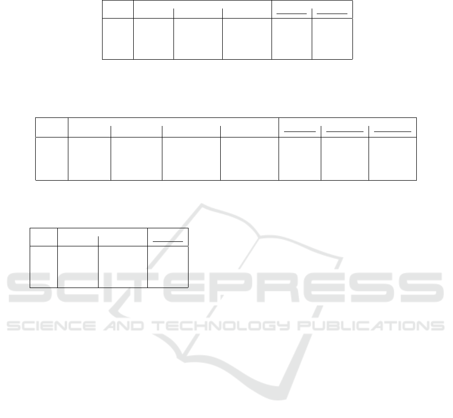
Table 3: Collision detection: Wall-clock times (reported in seconds) required to generate the list of incompatible test points.

The table compares the sequential, the multi-core CPU-based, and the many-core GPU-based versions.

#Tests Times [s] Speedups

Sequential Parallel CPU Parallel GPU

Sequential

Parallel CPU

Sequential

Parallel GPU

100 0.004 0.006 0.019 0.67 0.21

1,000 0.300 0.060 0.148 4.69 2.03

10,000 17.440 9.000 4.150 1.92 4.20

30,000 267.300 37.870 19.430 7.06 13.76

30,000

∗

191.140 59.750 46.510 3.20 4.11

Table 4: Distance computation: Wall-clock times (reported in seconds) required to compute the distance among all test point

pairs not contained in the incompatibility list. The comparison include the sequential version, the multi-core CPU approach,

and two many-core GPU-bases approaches (the ﬁrst one optimized for memory usage and the second one for computation

time).

#Tests Times [s] Speedups

Sequential Parallel CPU Parallel GPU

V 1

Parallel GPU

V 2

Sequential

Parallel CPU

Sequential

Parallel GPU

V 1

Sequential

Parallel GPU

V 2

100 0.004 0.006 0.019 0.008 0.69 0.21 0.50

1,000 0.300 0.110 0.148 0.071 2.69 2.03 4.23

10,000 17.440 3.544 4.150 0.860 4.92 4.50 20.78

30,000 267.300 52.255 19.430 3.630 7.06 13.75 73.64

30,000

∗

191.140 26.547 46.510 3.610 7.20 4.10 52.95

Table 5: Empirical time measurements and comparisons be-

tween single threaded and parallel pattern implementations

of the test planning.

#Tests Times [s] Speedups

Sequential Parallel CPU

Sequential

Parallel CPU

22 0.138 0.196 0.70

160 0.042 0.046 0.91

2156 43.330 18.950 2.29

5046 15.520 3.530 4.40

6507

∗

1084.260 447.26 2.42

its initial position and moving to the closest test point

at each step. It essentially applies a greedy “travel-

ing salesman problem” to our PCB problem in which

at each step the probe moves on the closest untested

point. In this case the algorithm is not suitable for

a GPU computation, as it is heavily based on the se-

lection of the next point. This selection would make

threads divergence too high and would slow down the

GPU computation.

6 CONCLUSIONS

In this paper, we describe a motion-planning applica-

tion in which 8 probes have to move over a printed cir-

cuit board to reach a sequence of test conﬁgurations.

We designed a low-level application optimizing the

steps required to move between those conﬁgurations

without the probes crossing each other. The solution

offers a trade-off between the computational time and

the probe repositioning time, ﬁnding a reliable local

solution for each probe and optimizing their simul-

taneous change of position for that movement. Al-

though the resulting path may result sub-optimal, ex-

perimental results show how the multi-core approach

effectively reduces the average path ﬁnding time by a

signiﬁcant amount.

Among the future work, we plan to produce a

board and a test-sequence generator to verify our tool

and make the software publicly available. Further

optimizations will be required on some speciﬁc and

collateral phases of the algorithm. More experiments

will also be in order with a tighter integration of the

new algorithmic features with the ones already used

by the test planner.

REFERENCES

Bonaria, L., Raganato, M., Reorda, M. S., and Squillero, G.

(2019a). A Dynamic Greedy Test Scheduler for Op-

timizing Probe Motion in In-Circuit Testers. In 2019

IEEE European Test Symposium (ETS), pages 1–2.

Bonaria, L., Raganato, M., Squillero, G., and Reorda, M. S.

(2019b). Test-Plan Optimization for Flying-Probes In-

Circuit Testers. In 2019 IEEE International Test Con-

ference in Asia (ITC-Asia), pages 19–24.

Coombs, C. F. (2016). Printed Circuits Handbook (7th Edi-

tion). McGraw-Hill, Inc., USA.

Dijkstra, E. W. et al. (1959). A note on two problems

in connexion with graphs. Numerische mathematik,

1(1):269–271.

Hiratsuka, Y., Katoh, F., Konishi, K., and Shin, S. (2010).

A Design Method for Minimum Cost Path of Flying

Probe In-Circuit Testers. In Proceedings of SICE An-

nual Conference 2010, pages 2933–2936.

Jurj, S. L., Rotar, R., Opritoiu, F., and Vladutiu, M.

(2020). Affordable Flying Probe-Inspired In-Circuit-

Tester for Printed Circuit Boards Evaluation with Ap-

plication in Test Engineering Education. In 2020

IEEE International Conference on Environment and

Electrical Engineering and 2020 IEEE Industrial and

Commercial Power Systems Europe (EEEIC / I CPS

Europe), pages 1–6.

ICSOFT 2021 - 16th International Conference on Software Technologies

292

Li, W., Yang, J., Lv, X., and Wang, J. (2020). A New

Path Planning Method for Flying Probe Test Arms. In

Chinese Control And Decision Conference (CCDC),

pages 1552–1556.

Radev, P. and Shirvaikar, M. (2006). Enhancement of Fly-

ing Probe Tester Systems with Automated Optical In-

spection. In Proceeding of the Thirty-Eighth South-

eastern Symposium on System Theory, pages 367–

371.

Soh Ying Seah, Melanie Po-Leen Ooi, Ye Chow Kuang,

Chee Sun See, Panchadcharam, S., and Demidenko,

S. (2009). Combining ATE and Flying Probe In-

Circuit Test Strategies for Load Board Veriﬁcation and

Test. In 2009 IEEE Instrumentation and Measurement

Technology Conference, pages 1380–1385.

van Schaaijk, H., Spierings, M., and Marinissen, E. J.

(2018). Automatic Generation of In-Circuit Tests for

Board Assembly Defects. In IEEE 23rd European Test

Symposium (ETS), pages 1–2.

Smart Techniques for Flying-probe Testing

293