Energy-based Control for Soft Manipulators

using Cosserat-beam Models

Brandon Caasenbrood

1 a

, Alexander Pogromsky

1,2 b

and Henk Nijmeijer

1 c

Department of Mechanical Engineering, Eindhoven University of Technology, The Netherlands

Department of Control Systems and Informatics, Saint-Petersburg National Research University of Information

Technologies, Mechanics, and Optics (ITMO), Russian Federation

Keywords:

Soft Robotics, Cosserat Beam Theory, Dynamic Modeling, Energy-based Control.

Abstract:

In this work, we describe an energy-based control method for under-actuated soft manipulators. The con-

tinuous dynamics of the soft robot are modeled by the differential geometry of Cosserat beams. Through a

ﬁnite-dimensional truncation, a reduced port-Hamiltonian model is obtained that preserves desirable passivity

conditions. Exploiting the passivity, we propose a stabilizing energy-shaping controller that ensures the poten-

tial energy is minimal at the desired end-effector conﬁguration. Finally, the effectiveness of the energy-based

controller is demonstrated through simulations of a soft manipulator inspired by the tentacle of an octopus.

1 INTRODUCTION

With an origin in material science, soft robotics is

slowly vesting itself as a prominent successor to con-

ventional rigid robotics. Unlike traditional robots,

soft robots are composed of ‘soft materials’ that en-

able a rich family of motion primitives, inherent

safety, and robustness towards environmental uncer-

tainties. By fully exploiting the properties in soft ma-

terials, soft robotics places the ﬁrst stepping stones to-

wards achieving performance similar to biology (Choi

et al., 2011; Falkenhahn et al., 2015; Marchese et al.,

2014; Kriegman et al., 2019). In this paper, we pri-

marily focus on a particular subclass of soft robotics

– soft robot manipulators.

Although signiﬁcant steps have been taken to-

wards bridging biology and soft robotics, its innate

inﬁnite-dimensionality poses substantial challenges

on modeling and control. In theory, soft robots pos-

sess inﬁnitely many degrees-of-freedom along their

continuously deformable body, rendering them partic-

ularly suited for Partial Differential models. Besides,

their mechanical design often employs distributed ac-

tuation (e.g., pneumatics and tendons). Classical de-

scriptions of rigid links and joints paired with lo-

calized actuation are therefore no longer viable nor

https://orcid.org/0000-0002-6299-1730

https://orcid.org/0000-0001-8755-9832

https://orcid.org/0000-0001-5883-6191

physically representative. This paradigm shift calls

for new control-oriented modeling approaches suited

for these intrinsically hyper-redundant and under-

actuated robotic systems.

In the last decade, modeling approaches for soft

robot manipulators have matured sufﬁciently and as

such their applicability in model-based control is

slowly realizable. To highlight a few: reduced-

order ﬁnite element models (Duriez, 2013; Zhang

et al., 2017), constant and non-constant curvature ap-

proaches (Katzschmann et al., 2019; Della Santina

and Rus, 2020), Cosserat-beam models (Renda et al.,

2020; Boyer et al., 2020), modal approximations

(Chirikjian and Burdick, 1992), and learning-based

approaches (Thuruthel et al., 2018). Among them,

the Piece-wise Constant Curvature (PCC) model re-

mains one of the most favored techniques of spa-

tial reduction. The PCC model has proven to be

viable for applications like feedforward controllers

(Falkenhahn et al., 2015), and more recently feedback

dynamic controllers (Della Santina and Rus, 2020;

Katzschmann et al., 2019). Nevertheless, the ap-

proach has its limitations. They do not originate from

continuum mechanics and thus are only applicable in

restrictive settings. Although they offer better compu-

tationally performance than continuous models, due

to their kinematic restrictions, they are unable to cap-

ture important continuum phenomena, like buckling,

environmental interaction or wave propagation.

Caasenbrood, B., Pogromsky, A. and Nijmeijer, H.

Energy-based Control for Soft Manipulators using Cosserat-beam Models.

DOI: 10.5220/0010581503110319

In Proceedings of the 18th International Conference on Informatics in Control, Automation and Robotics (ICINCO 2021), pages 311-319

ISBN: 978-989-758-522-7

311

Cosserat beam-models, on the other hand, have

shown to capture a wider range of nonlinear contin-

uum deformations. These models are rooted in con-

tinuum mechanics and thus provide a more accurate

description of the hyper-ﬂexible nature of soft robots.

The computational dynamics of Cosserat beams have

been extensively developed by (Simo and Vu-Quoc,

1986)through Geometrically-Exact ﬁnite elements on

the Lie group SE(3); and recently, these models are

slowly gaining popularity in the soft robotics commu-

nity (Renda et al., 2020; Boyer et al., 2020; Till et al.,

2019). Ultimately, the strong nonlinearities paired

with the diligence to achieve biological performance

encourage Cosserat models for feedback control. Yet,

to the author’s knowledge, their application on model-

based feedback control is relatively scarce.

In this work, we aim to highlight the capabilities

of Cosserat models for model-based control, in par-

ticular energy-based strategies. To this end, a ﬁnite-

dimensional modeling approach is proposed such that

the continuous dynamics can be cast into a port-

Hamiltonian (pH) structure. The main advantage of

pH systems is the common formalism with energy-

based control. Through the pH structure, we pro-

pose an energy-shaping control law that ensures sta-

bilization of the end-effector of the soft robot. Sim-

ilar energy-based control strategies can be found in

(Franco and Garriga-Casanovas, 2020; Schaft, 2004;

Ortega et al., 2002) for rigid-body systems. As a study

case, we consider a soft robot manipulator inspired by

an octopus tentacle (see Figure 1). With the ability to

deform continuously and its distributed muscular sys-

tem, it is ideal for illustrating the complex morpholog-

ical motions present in soft robotics. All source code

is made publicly available at (Caasenbrood, 2020).

The paper is organized as follows. Section 2 will

detail a modeling approach for a general class of soft

robot manipulators, starting with the Cosserat-beam

theory. In Section 3, we propose an energy-shaping

control strategy. Lastly, we show the effectiveness

of energy-based controller through numerical simu-

lation, followed by a brief conclusion in Section 5.

2 DYNAMIC MODELING

2.1 Lie Group Notations

Throughout this work, we will explore Lie group the-

ory. We introduce the following notations: the Lie

group of rigid-body transformation on R

is denoted

by SE(3), whereas the group of homogeneous rota-

tion is denoted by SO(3). The tangent space at the

identity of the group is called the Lie algebra, and it

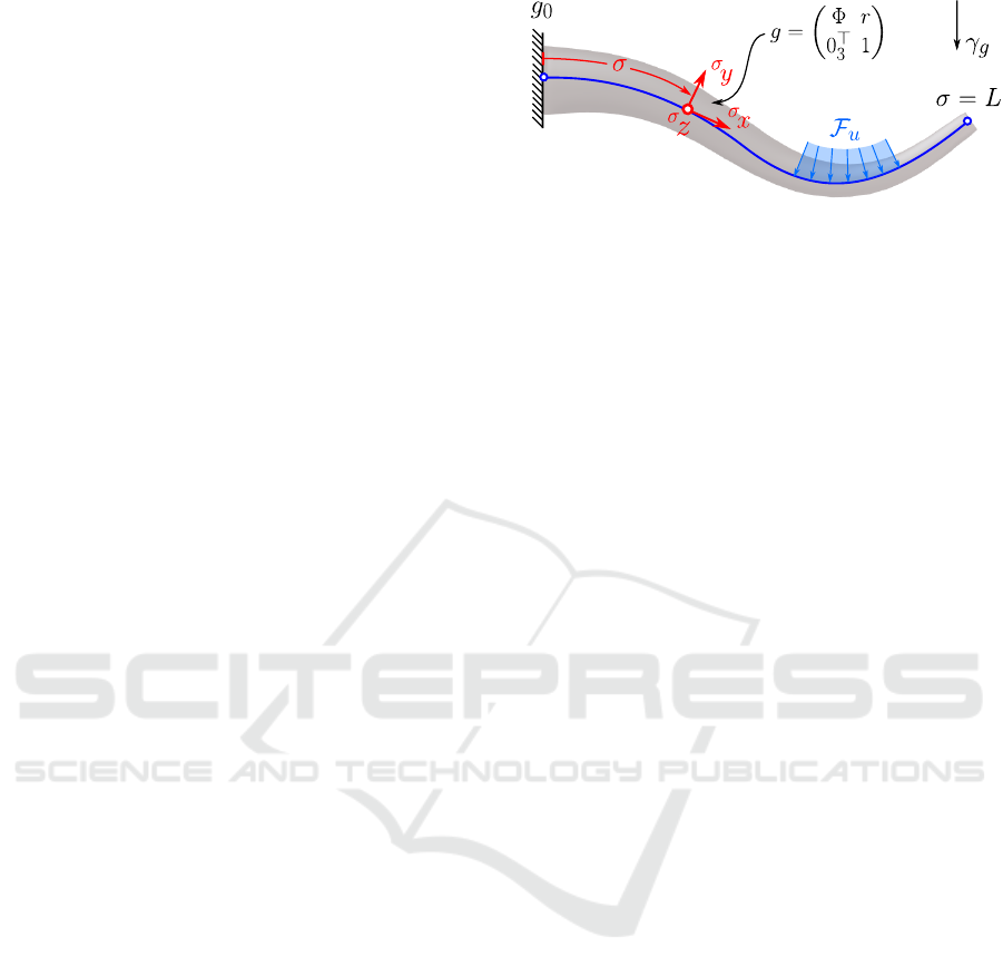
Figure 1: Schematic representation of a soft robot manipu-

lator inspired by the tentacle of an octopus. The soft robot

is model as a Cosserat beam with distributed actuation F

can be used to describe the evolution of the Lie group.

The Lie algebra of SE(3) and SO(3) are denoted by

se(3) and so(3), respectively. Lastly, the cross opera-

tor (i.e., ”×”) and hat operator (i.e., ”∧”) are used to

transform a column vector of R

or R

into an ele-

ment of the Lie algebra so(3) or se(3), respectively.

2.2 Cosserat Beam Theory

In Cosserat theory, slender deformable solids are

modeled as elastic strings subjected to geomet-

ric ﬁnite-strain theory. Drawing the analogy to

soft robotics, we model the soft robot as a one-

dimensional spatial curve passing through the geo-

metric center of the soft robot (see Figure 1). We

call this curve the ’backbone curve’. Given its spatial-

temporal nature, we introduce a temporal variable t ∈

[0, T ] with ﬁnite horizon time T , and a spatial variable

σ ∈ [0, L] with L the undeformed length of the soft

robot. For convenience, we denote T = [0, T ] and X =

[0, L]. For each point on the backbone, we introduce

a (mobile) Serret-Frenet frame that is spanned by a

basis of orthonormal vectors {

z}. The homo-

geneous rotation related to these Serret-Frenet frames

is given by the rotation matrix Φ(σ,t) ∈ SO(3), and

their origin by the position vector r(σ,t) ∈ R

Following the geometric approach (Simo and

Vu-Quoc, 1986; Boyer et al., 2010; Renda et al.,

2020), we may equivalently represent all Serret-

Frenet frames that are rigidly attached to the continu-

ous backbone by a parameterized curve in SE(3):

g(σ,t) :=



Φ(σ,t) r(σ,t)



∈ SE(3). (1)

By considering the partial derivatives of g, an expres-

sion for the strain ﬁeld ξ and velocity ﬁeld η any-

where on the Cosserat beam can be found in terms of

its Lie algebra se(3). To do so, we have to introduce

some smoothness conditions:

Assumption 1. All control inputs, i.e., a distributed

control wrench acting on the system, are considered to

be sufﬁciently smooth for any instance t ∈ T and σ ∈

ICINCO 2021 - 18th International Conference on Informatics in Control, Automation and Robotics

312

X such that the resulting backbone g(σ,t) ∈ SE(3) is

everywhere differentiable.

2.3 Local Strain and Velocity

Let Γ = (κ

, κ

,κ

)

and U = (ν

, ν

)

be the

torsion-curvature and elongation-shear strain vector,

respectively. Then, an expression for strain ﬁeld

ξ(σ,t) is obtained through spatial differentiation of g:

ξ := g

−1

∂g

∂σ

=⇒ ξ :=





, (2)

Similarly, let Ω = (ω

,ω

)

and V = (v

, v

)

be the angular and linear velocity vector, respectively.

Then, an expression for velocity ﬁeld η(σ,t) is ob-

tained through time differentiation of g:

η := g

−1

∂g

∂t

Ω

=⇒ η :=



Ω



. (3)

Since we assume g to be everywhere differentiable,

we can derive a PDE relation for the continuous for-

ward kinematics of the soft robot:

∂η

∂σ

= −ad

η +

ξ, (4)

where ad

(·)

: R

7→ R

6×6

denotes the adjoint action

on the Lie algebra (full derivation in Appendix A).

For completeness, we introduce the adjoint action on

the group and its algebra by



Φ 0

Φ Φ



; ad





, (5)

respectively. Drawing an analogy to rigid robotics,

the expression in (4) may be seen as the forward ve-

locity kinematics for a serial chain robot manipulator

with inﬁnitely many links. The expressions for the

Cosserat beam kinematics above is derived similarly

in (Boyer et al., 2020) and (Renda et al., 2020).

2.4 Finite-dimensional Reduction

Similar to ﬁnite element methods, we wish to ﬁnd

a ﬁnite-dimensional approximation of the strain ﬁeld

ξ(σ,·) for all points on the material domain X. To do

so, we assume the following:

Assumption 2. Any element of the strain ﬁeld ξ(σ,t)

can be written as an inﬁnite expansion of the follow-

ing form:

(σ,t) =

∞

∑

n=1

(σ)q

i,n

(t) + ξ

◦

(σ) i ∈ {1, ... ,6},

(6)

where {θ

}

∞

n=1

is the set of basis functions θ

: X → R

together with modal coefﬁcients q

i,n

: T → R , and an

intrinsic time-invariant strain ξ

◦

: X → R . The basis

functions θ

(·) and the modal coefﬁcients q

(·) are

both smooth functions.

Assumption 3. Given (6), the k-th order truncation

for an element of the strain ﬁeld, deﬁned as

[ξ

]

(σ,t) :=

∑

n=1

(σ)q

i,n

(t) +ξ

◦

(σ) i ∈ {1,. .., 6},

(7)

converges uniformly on T and X as the index k → ∞.

Moreover, we assume that uniform convergence holds

for its partial derivatives

∂

∂t

[ξ]

and

∂

∂σ

[ξ]

Accordingly, we can rewrite the k-th order truncation

of the complete strain ﬁeld as follows

[ξ]



⊗



.. . θ



q + ξ

◦







.. . θ

.. . 0 ·· · 0

0 · ·· 0 .. . θ

.. . θ







{z }

Θ(σ)







1,1

6,k







+ ξ

◦

, (8)

where Θ ∈ R

6×6k

is a sparse shape function matrix

with mutually orthogonal columns, the operator ⊗ de-

notes the Kronecker product, and the vector q ∈ R

is the collection of all time-variant modal coefﬁcients.

Although a wide variety of bases are possible (Boyer

et al., 2020; Della Santina and Rus, 2020), we have

chosen a modiﬁed Legendre polynomial set:

(σ) =

(n − 1)!

n−1

dσ

n−1



2σ

− 1



− 1

n−1

(9)

with n ∈ Z

the polynomial degree. An alternative

option could be constructing the set of basis func-

tions through the so-called ’snapshot decomposition

method’ using FEM-driven data (Astrid et al., 2008).

2.5 Finite-dimensional Kinematics

Given the ﬁnite-dimensional truncation in (8), we can

now ﬁnd an expression for the ﬁnite-dimensional for-

ward kinematics in terms of the generalized coordi-

nates q and its velocities components ˙q.

First, let us regard the conﬁguration of the soft

robot g ∈ SE(3). Recall that the spatial evolution of

the conﬁguration is described by ∂g/∂σ = gξ

∧

, see

Eq. (2). Given the initial condition g(0, ·) = g

, an

approximation of the continuously deformable soft

robot can be obtained by partial integration over the

spatial domain:

[g]

(σ,t) = g

[

ξ]

(s,t) ds. (10)

Energy-based Control for Soft Manipulators using Cosserat-beam Models

313

Next, lets regard the velocity kinematics η(σ,t) for

any point σ on the backbone curve. Using the

differential property of the adjoint action ad

−∂/∂σ[Ad

−1

]Ad

(Murray et al., 1994), we can

rewrite the continuous forward kinematics in (4) as

∂η

∂σ

∂

∂σ



−1



η +

ξ. (11)

Now, given the initial condition η(0, ·) = 0

and the

approximations [ξ]

and [g]

, we can ﬁnd an approx-

imation to the velocity twist η by partial integration

over space:

[η]

(σ,t) = Ad

−1

[g]

Θ ds ˙q := [J]

˙q, (12)

which naturally gives rise to the geometric Jacobian

[J]

∈ R

6×6k

. The geometric Jacobian plays an im-

portant role in obtaining the Lagrangian form of the

reduced-order dynamic model. Finally, to express the

acceleration twist, we take the time-derivative of (12)

leading to

[

η]

= [J]

¨q +

[J]

˙q,

= [J]

¨q + Ad

−1

[g]

[η]

Θ ds ˙q, (13)

which gives rise to the analytic expression of the time-

derivative of the geometric Jacobian

[J]

(see Ap-

pendix B for the derivation).

2.6 Finite-dimensional Dynamics

Here, we detail the dynamics of the Cosserat beam.

First, let us consider an inﬁnitesimal slice of con-

tinuum body that is perpendicular to the backbone

curve. The kinetic momenta of this inﬁnitesimal slice

is then given by µ(σ,t) = M η(σ,t) in which M ∈

∗

(3) × se(3)

∼

6×6

denotes the symmetric inertia

tensor.

Remark 1. For some soft robots, the inertia tensor

M may have an explicit dependency on space or time

(or both). Nevertheless, for sake of simplicity, we limit

ourselves to a diagonal invariant inertia tensor M =

diag

{

ρI

,ρA

}

with line-density ρ > 0 and the second

moment of area A ∈ so

∗

(3) × so(3)

∼

3×3

Using the expression of the kinetic momenta µ of the

inﬁnitesimal body, we can write the equation of mo-

tion for a particular slice at σ using the Newton-Euler

equations:

∂

∂t

(Ad

−>

µ) = Ad

−>

F , (14)

where again Ad

(·)

stands for the adjoint action on

the Lie group, and F = F

+ F

− F

the resul-

tant wrench that is composed of the constraint wrench

, the input wrench F

, and the potential wrenches

due to gravity and visco-elasticity, F

and F

, respec-

tively. Further evaluation of (14) leads to

η − ad

M η = F , (15)

where we used the fact that

−1

= −ad

−1

. Be-

fore continuing, we introduce a slight modiﬁcation to

the relation above. Using the fact that ad

η = 0

, we

can introduce the vector M ad

η to (15) without af-

fecting the dynamics. The importance of this modiﬁ-

cation originates from the preservation of passivity in

the Lagrangian model, which is an important property

in stability theorems for robotics. By substitution of

the null vector, the equation of motion becomes

η +



M ad

− ad



η = F , (16)

which is nothing more than the Newton-Euler equa-

tion for rigid-body motion on R

. To introduce the

(reduced-order) Cosserat kinematics and make the ex-

pression symmetric, we substitute (12) and (13) into

(16) and pre-multiply by [J ]

[J ]



M [J ]

¨q + M [

J ]

˙q + C

[η ]

˙q



= [J ]

− F

), (17)

where C

(·)

= −C

(·)

:= M ad

(·)

− ad

(·)

M is a skew-

symmetric matrix. It is important to note that by

pre-multiplication of the transpose Jacobian, we have

eliminated the constraint wrenches, i.e., [ J ]

= 0

(Murray et al., 1994). Finally, the ﬁnite-dimensional

dynamics of the deformable soft robot is found by

spatial integration of (16) over the material domain

X. The overall dynamics can be written in familiar

Euler-Lagrangian (EL) form as follows

M(q) ¨q +C(q, ˙q) ˙q + N(q) + F(q, ˙q) = τ(q,t) (18)

with the system matrices:

M(q) =

[J ]

M [J ]

dσ, (19)

C(q, ˙q) =

[J ]

M [

+ [ J ]

[η]

[J]

dσ, (20)

N(q) =

[J]

dσ, (21)

F(q, ˙q) =

[J]

dσ := Kq + D ˙q, (22)

τ(q,t) =

[J]

dσ := Gu(t), (23)

where M is the generalized inertia matrix, C the

centripetal-Coriolis matrix, N a vector of generalized

potential forces with F

= −Ad

−1

[g]

M γ

the external

wrench acting on the body due to gravitational accel-

eration γ

, and F

a vector of viscoelastic forces im-

posed by the stiffness matrix K and damping matrix

ICINCO 2021 - 18th International Conference on Informatics in Control, Automation and Robotics

314

D. The vector Gu represents the distributed forces

and torques generated by various kinds of the internal

actuators (e.g., tendons or pneumatics). If rank(G) <

dim(q), the system is considered to be under-actuated.

Within the context of soft robotics, whose inﬁnite-

dimensional conﬁguration space cannot be matched

by a ﬁnite number of actuators, these systems are of-

ten intrinsically under-actuated. Following the pro-

cedures in ﬁnite elements and assuming linear vis-

coelasticity, the stiffness matrix and damping matrix

are computed through spatial integration:

K =

K Θ dσ, (24)

D =

D Θ dσ, (25)

where K ∈ se

∗

(3)× se(3) and D ∈ se

∗

(3)× se(3) are

the stiffness and damping tensor, respectively.

Lemma 1. The inertia matrix M(q) is a symmet-

ric, positive deﬁnite, symmetric. and is uniformly

bounded such that there exists constants λ

< λ

such

that λ

(q)I

 M(q)  λ

(q)I

< ∞.

Proof. Proof can be found in (Spong et al., 2006)

Lemma 2. Given the inertia matrix M(q) and the

Coriolis matrix C( ˙q,q) as described by (19) and (20),

respectively, it can be shown that the matrix

M − 2C

is skew-symmetric.

Proof. To show

M − 2C is skew-symmetric, we start

by computing the time-derivative of the inertia matrix.

For sake of clarity, lets abbreviate [J ]

= J and [

J ]

J. Through chain differentiation, we ﬁnd

M =

M J + J

J dσ, (26)

Then, calculating

M −2C leads to

M −2C =

M J − J

J − 2J

C J dσ. (27)

Since J

C J is skew-symmetric, the remainder of

the proof consists of showing that the matrix S =

M J − J

J also satisﬁes skew-symmetry. Since

M = M

, we can easily show this holds true:

S =

J − J

= −



J − J



= −S

. (28)

Therefore, the matrix

M −2C is skew-symmetric.

In literature, Lemma 2 is often referred to as the

passivity condition. It implies that, in the absence

of external dissipation, the total energy of the system

(i.e., the Hamiltonian) is conserved. It shall be clear

that the passivity property is an important means of

proving stability for robotic systems. It is also worth

mentioning that this condition does not necessarily

hold true for all cases, only for particular computa-

tions of the Coriolis matrix C(q, ˙q) (e.g., through the

Christoffel symbols).

2.7 port-Hamiltonian Formulation

In this section, the Lagrangian model in (18) is rewrit-

ten in port-Hamiltonian form. To this end, we de-

ﬁne the generalized momenta p := M ˙q. Then, the

(reduced-order) Hamiltonian is given by H = T + V

with T (p, q) =

−1

p and V (q) the kinetic and

potential energy of reduced system, respectively.

Given the Hamiltonian H , it can be easily shown

that generalized velocities can be written in terms of

partial derivatives of the Hamiltonian function

˙q =

∂H

∂p

= M

−1

p. (29)

Note that M

−1

exists due to the positive deﬁniteness

condition in Lemma 1. Similarly, we aim to ﬁnd a

differential equation that relates the time evolution of

p to the Hamiltonian. Applying the chain rule of dif-

ferentiation to the generalized momenta p, we ﬁnd

˙p =

M ˙q + M ¨q,



M −C − D



−1

p − Kq − N + Gu, (30)

Taking the partial derivate of the Hamiltonian H with

respect to the generalized coordinates q, we ﬁnd

∂H

∂q

∂

∂q



˙q

M(q) ˙q



∂V

∂q

. (31)

To relate (30) and (31), we have to exploit some struc-

tural properties in the Lagrangian model. To be more

speciﬁc, we exploit the skew-symmetry condition as

detailed in Lemma 2. According to the (Spong et al.,

2006), if the matrix S =

M − 2C satisﬁes the passivity

condition in Lemma 2, it can be shown that

S ˙q = −

∂

∂q



˙q

M(q) ˙q



−

M ˙q. (32)

Finally, by combining (29), (30), (31), and (32), we

can show that the Lagrangian model in (18) can be

equivalently rewritten as a port-Hamiltonian system:











˙q =

∂H

∂p

˙p = −

∂H

∂q

− D

∂H

∂p

+ Gu.

(33)

with the reduced-order Hamiltonian H =

−1

V . The advantage of the port-Hamiltonian model

over the EL structure in (18) is the general applica-

bility to different physical domains and the common

formalism with energy-based control techniques.

Energy-based Control for Soft Manipulators using Cosserat-beam Models

315

3 ENERGY-BASED CONTROL

In this section, we aim to ﬁnd a control law u that

ensures lim

t→∞

g(L,t) = g

where g

∈ SE(3) de-

notes the desired conﬁguration of the end-effector.

To achieve the control objective, the idea is to shape

the potential energy of the reduced-order dynamical

system using conventional energy-shaping techniques

from the port-Hamiltonian control theory.

3.1 Energy-shaping Controller

We adopted an energy-based control strategy akin

to the work of (Ortega et al., 2002) and (Franco

and Garriga-Casanovas, 2020). Following a simi-

lar energy-shaping strategy, the nonlinear controller

takes the form

u = G



∂H

∂q

−

∂H

∂q



, (34)

where G





−1

is the generalized inverse

of G, and H

−1

p + V

denotes the desired

Hamiltonian of the closed loop system that satisﬁes

argmin

= g

with g

= g(L,·). Note that we

omitted any damping injection since the material’s

intrinsic viscoelastic damping is deemed sufﬁciently

large to guarantee stability. Following the concept of

a kinematic feedback controller that artiﬁcially mim-

ics an elastic element between the end-effector and

the desired conﬁguration in SE(3), we choose the

variation of the desired potential energy as follows

= λ



+ λ



−1

, (35)

where λ

> 0 is a proportional gain, λ

> 0 a con-

troller gain related to the damping of the pseudo-

inverse, F

= k

log

SE(3)

([g

]

−1

) an artiﬁcial con-

trol wrench with positive deﬁnite matrix k

, and

log

SE(3)

: SE(3) 7→ se(3) the logarithmic map. The

controller gains λ

and λ

can be tuned accordingly

to tweak the desired transient behavior of the closed-

loop system, similar to a classical PD controller.

4 NUMERICAL STUDY CASE

In this section, we detail some numerical simulations

using the proposed dynamic model in (33) together

with the energy-shaping controller in (34). The trun-

cation degree of the ﬁnite-dimensional model is k = 8.

To simulate the under-actuation, we assume an input

matrix G = blkdiag

{

}

such that only the ﬁrst

three modes are actively controllable.

Table 1: Parameters setting for the numerical solver, the soft

manipulator, and the energy-based controller.

Parameter description Value

Undeformed length L = 120 (mm)

Density ρ = 1250 (kgm

−3

)

Gravitational acceleration γ

= 9.8 (ms

−2

)

Young’s modulus E = 25 (MPa)

Shear modulus µ

= 10 (MPa)

Constraint modulus µ

= 15 (GPa)

Rayleigh coefﬁcient ζ = 0.4 (-)

Due to the partial differential nature, we have to

employ a nested ODE routine to recover the trajecto-

ries for q and p. First, we employ an implicit trape-

zoidal solver with a ﬁxed timestep of dt = 1 ms to

solve (33). At each time increment, we have to eval-

uate the dynamic matrices (17)-(22). To efﬁciently

compute these dynamic entities, we solve the spatial

integration problem over the material domain X by

using a second-order Runge-Kutta solver. The step-

size for the spatial solver is dσ = 1 mm. The open-

source code is written in c++ and MATLAB, which is

made publicly available at (Caasenbrood, 2020)

For soft material parameters, we choose an

isotropic Hookean material with shear constraints.

All the material properties related to the soft material

are provided in Table 1. Given these material proper-

ties, the inertia tensor and the stiffness tensor become

diagonal matrices:

M = blkdiag

{

ρA, ρA, ρA, ρA

}

K = blkdiag

{

A, EA, µ

A, µ

}

where A > 0 is the (average) cross-sectional area, and

A the second moment of area for a circular disc with

radius R = 8 mm. The damping tensor is chosen as

D = ζK with damping coefﬁcient ζ. The general-

ized stiffness and damping matrix can then be pre-

computed using (23) and (24).

As for control settings, the control gains are tuned

to produce a smooth transient: λ

= 0.1 and λ

0.01. The artiﬁcial spring stiffness is chosen as k

blkdiag

{

0.01 · I

}

. Lastly, the desired conﬁgura-

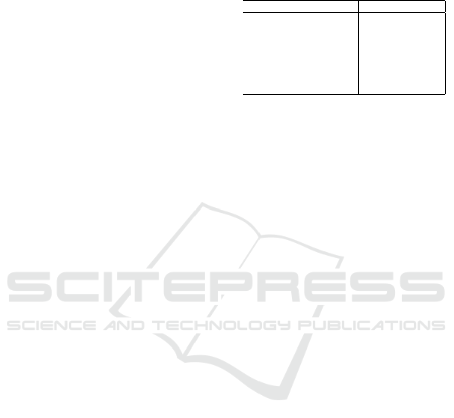
tion of the end-effector is chosen as follows:





with r





0.05

0.00

−0.01





The simulation results for the closed-loop soft

robotic system are shown in Figure 2 and Figure

3. Figure 2 shows the trajectories of the modal co-

efﬁcients q(t) and the spatial trajectory of the end-

effector of the soft robot, whereas Figure 3 has been

provided to show the evolution of the continuous de-

formation of the soft robot. As can be seen, the

ICINCO 2021 - 18th International Conference on Informatics in Control, Automation and Robotics

316

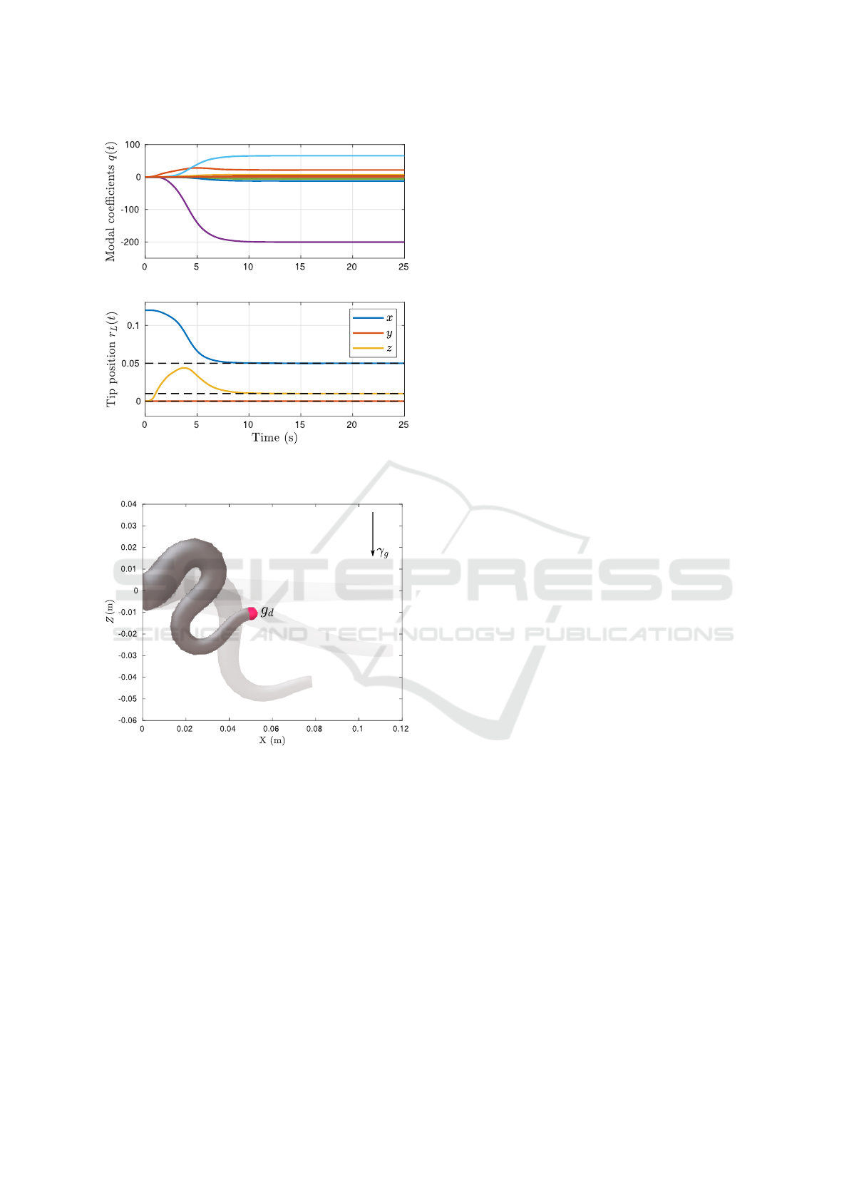
Figure 2: The evolution of the modal coefﬁcients and the

position of the end-effector of the soft robot manipulator.

Figure 3: Three-dimensional evolution of the soft robot

manipulators, slowly converging to the desired set-point

∈ SE(3).

end-effector of the soft robot manipulator slowly con-

verges to the desired set-point g

∈ SE(3). Although

the control gains could be increased to promote a

faster transient, it was observed that high gains lead

to signiﬁcant oscillations of the ﬂexible structure.

A possible solution might be to introduce negative

damping to the controller Hamiltonian H

, to over-

come the soft robot’s structural damping.

5 CONCLUSION

The ﬁeld of soft robotics is slowly maturing into a

recognized subﬁeld of robotics. Due to their intrin-

sic compliance, they allow for complex morphologi-

cal motions that mimic animals in nature. Achieving

similar performance to biology highlights the need

for more accurate dynamic models and control strate-

gies that fully exploit the hyper-redundant nature of

soft robots. In this work, we provided a modeling

framework for Cosserat beams that leads to a ﬁnite-

dimensional system in a port-Hamiltonian structure.

By exploiting the passivity, an energy-shaping con-

troller was proposed that ensures the closed-loop

Hamiltonian is minimal at the desired set-point. In-

spired by an octopus, a numerical model was devel-

oped for a tentacle-like soft robot with distributed

control inputs. The key challenges here regarding

both the model as the controller are their ability

to capture the hyper-ﬂexibility, deal with intrinsic

under-actuation, and exploit its hyper-redundancy to

achieve its control task. Given appropriate controller

gains, the model-based controller yields smooth con-

vergence of the soft robot’s end-effector while ac-

counting for the intrinsic underactuated nature. More-

over, the mobility of the Cosserat model paired with

the energy-based control has, to some extent, a resem-

blance to the biological motions seen in octopuses.

Future work will focus on the following: i) validat-

ing the model and the controller experimentally, ii)

adding hyper-elasticity, iii) constructing a set of basis

functions through the so-called ’snapshot’ decompo-

sition method using FEM-driven data. In particular,

the latter goal could be interesting to explore both ad-

vantages in FEM and Cosserat models, being accu-

rate continuum deformations and computational efﬁ-

ciency, respectively.

ACKNOWLEDGEMENTS

This work is partly supported by NWO, Netherlands

Organization for Scientiﬁc Research; and is part of

the Wearable Robotics perspective program. Website:

www.wearablerobotics.nl.

REFERENCES

Astrid, P., Weiland, S., Willcox, K., and Backx, T. (2008).

Missing point estimation in models described by

proper orthogonal decomposition. IEEE Transactions

on Automatic Control, 53(10):2237–2251.

Energy-based Control for Soft Manipulators using Cosserat-beam Models

317

Boyer, F., Lebastard, V., Candelier, F., and Renda, F. (2020).

Dynamics of continuum and soft robots: a strain

parametrization based approach. IEEE Transactions

on Robotics.

Boyer, F., Porez, M., and Leroyer, A. (2010). Poincar

cosserat equations for the lighthill three-dimensional

large amplitude elongated body theory: Application

to robotics. 20(1):47–79.

Caasenbrood, B. (2020). Sorotoki - an open-

source soft robotics toolkit for matlab.

https://github.com/BJCaasenbrood/SorotokiCode.

Chirikjian, G. and Burdick, J. (1992). Kinematically

optimal hyper-redundant manipulator conﬁgurations.

Proceedings 1992 IEEE International Conference on

Robotics and Automation.

Choi, W., Whitesides, G. M., Wang, M., Chen, X., Shep-

herd, R. F., Mazzeo, A. D., Morin, S. A., Stokes,

A. A., and Ilievski, F. (2011). Multigait soft robot.

Proceedings of the National Academy of Sciences,

108(51):20400–20403.

Della Santina, C. and Rus, D. (2020). Control oriented mod-

eling of soft robots: The polynomial curvature case.

IEEE Robotics and Automation Letters, 5(2):290–298.

Duriez, C. (2013). Control of elastic soft robots based on

real-time ﬁnite element method. Proceedings - IEEE

International Conference on Robotics and Automa-

tion, pages 3982–3987.

Falkenhahn, V., Mahl, T., Hildebrandt, A., Neumann,

R., and Sawodny, O. (2015). Dynamic Modeling

of Bellows-Actuated Continuum Robots Using the

Euler-Lagrange Formalism. IEEE Transactions on

Robotics, 31(6):1483–1496.

Franco, E. and Garriga-Casanovas, A. (2020). Energy-

shaping control of soft continuum manipulators with

in-plane disturbances. International Journal of

Robotics Research.

Katzschmann, R. K., Della Santina, C. D., Toshimitsu, Y.,

Bicchi, A., and Rus, D. (2019). Dynamic motion

control of multi-segment soft robots using piecewise

constant curvature matched with an augmented rigid

body model. RoboSoft 2019 - 2019 IEEE Interna-

tional Conference on Soft Robotics, (February):454–

461.

Kriegman, S., Blackiston, D., Levin, M., and Bongard, J.

(2019). A scalable pipeline for designing reconﬁg-

urable organisms.

Marchese, A. D., Onal, C. D., and Rus, D. (2014). Au-

tonomous Soft Robotic Fish Capable of Escape Ma-

neuvers Using Fluidic Elastomer Actuators. Soft

Robotics, 1(1):75–87.

Murray, R. M., Sastry, S. S., and Zexiang, L. (1994). A

Mathematical Introduction to Robotic Manipulation.

CRC Press, Inc., USA, 1st edition.

Ortega, R., Spong, M. W., G

omez-Estern, F., and Blanken-

stein, G. (2002). Stabilization of a Class of Under-

actuated MechanicalSystems Via Interconnection and

DampingAssignment. IEEE Transactions on Auto-

matic Control, 47(8):1218–1233.

Renda, F., Armanini, C., Lebastard, V., Candelier, F., and

Boyer, F. (2020). A Geometric Variable-Strain Ap-

proach for Static Modeling of Soft Manipulators with

Tendon and Fluidic Actuation. IEEE Robotics and Au-

tomation Letters, 5(3):4006–4013.

Schaft, A. J. (2004). Port-Hamiltonian Systems: Network

Modeling and Control of Nonlinear Physical Systems.

Advanced Dynamics and Control of Structures and

Machines, pages 127–167.

Simo, J. C. and Vu-Quoc, L. (1986). A three-dimensional

ﬁnite-strain rod model. part II: Computational aspects.

Computer Methods in Applied Mechanics and Engi-

neering, 58(1):79–116.

Spong, M. W., Hutchinson, S., and Vidyasagar, M. (2006).

Robot modeling and control. John Wiley & Sons, New

York.

Thuruthel, T., Falotico, E., Renda, F., and Laschi, C. (2018).

Model-based reinforcement learning for closed-loop

dynamic control of soft robotic manipulators. IEEE

Transactions on Robotics, PP:1–11.

Till, J., Aloi, V., and Rucker, C. (2019). Real-Time Dynam-

ics of Soft and Continuum Robots based on Cosserat-

Rod Real-Time Dynamics of Soft and Continuum

Robots based on Cosserat-Rod Models. (May).

Zhang, Z., Morales Bieze, T., Dequidt, J., Kruszewski, A.,

and Duriez, C. (2017). Visual Servoing Control of

Soft Robots based on Finite Element Model. In IROS

2017 - IEEE/RSJ International Conference on Intelli-

gent Robots and Systems, Vancouver, Canada.

APPENDIX

A. Deriving the Continuous Kinematics

Under Assumption 1, the conﬁguration space of the

soft robot g is everywhere differentiable. Then, using

the equality of mixed partials, i.e.

∂

∂t

(

∂g

∂σ

) =

∂

∂σ

(

∂g

∂t

we substitute ∂g/∂t = g

η and ∂g/∂σ = g

ξ to ﬁnd

ξ + g

∂

∂t

= g

η + g

∂

∂σ

. (36)

Pre-multiplying with g

−1

∈ SE(3) and rearranging the

equality above, we obtain

∂

∂σ

= −



η −



ξ, (37)

where we can recognize the Lie bracket or the com-

muter between the vector ﬁelds ξ and η (Murray et al.,

1994). Since the Lie bracket [

ξ,

η] itself also belongs

to se(3), which is isomorphic to R

via

η 7→ η, we

can rewrite the expressions as follows

∂η

∂σ

= −ad

η +

ξ, (38)

where ad

(·)

: R

7→ R

6×6

deﬁnes the adjoint action

map on the Lie algebra se(3). This kinematic relation

is analogous to (Boyer et al., 2020; Renda et al., 2020;

Till et al., 2019)

ICINCO 2021 - 18th International Conference on Informatics in Control, Automation and Robotics

318

B. Partial Derivative of the Geometric

Jacobian Matrix

The mapping from generalized coordinates ˙q ∈ R

the velocity-twist vector

η = g

−1

˙g ∈ se(3)

∼

for

a point σ be given by η = J ˙q where J is the geomet-

ric Jacobian. The k-th order truncations of the exact

geometric Jacobian is given by

[J]

= Ad

−1

[g]

Θ dσ. (39)

Again, Ad

(·)

above denotes the adjoint action on

SE(3). Unlike its notation in rigid robotics, note that

the geometric Jacobian matrix here is time and space-

variant. Following the chain rule of differentiation,

the partial time-derivate of the geometric Jacobian

matrix yields

[J]



−1

[g]



[g]

Θ dσ

+ Ad

−1

[g]



[g]



Θ dσ. (40)

Given the differential relations of the adjoint action

mapping on the Lie group, that is, d/ds (Ad

) =

given a twist ϒ = (g

−1

dg/ds)

∨

, we can ex-

press the time-derivate of the adjoint action and its

inverse as

∂

∂t

(Ad

) = Ad

, (41)

∂

∂t



−1



= −ad

−1

. (42)

Substituting the truncated variations of (41) and (42)

into (40), we ﬁnd the complete expression of the time-

derivate of the geometric Jacobian matrix

[J]

= −ad

[J]

+ Ad

−1

[g]

[η]

Θ dσ. (43)

Since ad

(J ˙q) = ad

η = 0

by deﬁnition, the ﬁrst

right-hand term vanishes if (43) is post-multiplied

with the generalized velocities ˙q, thus leading to the

expression for the acceleration twist

[η]

in (13).

Energy-based Control for Soft Manipulators using Cosserat-beam Models

319