Towards an Approach for Translation Validation of Thread-level

Parallelizing Transformations using Colored Petri Nets

Rakshit Mittal

1,2 a

, Rochishnu Banerjee

1 b

, Dominique Blouin

2,3 c

and Soumyadip Bandyopadhyay

1,3 d

Birla Institute of Technology and Science Pilani, KK Birla Goa Campus, Goa, India

Telecom Paris, Institut Polytechnique de Paris, Paris, France

Hasso Plattner Institut, Potsdam, Germany

Keywords:

Translation Validation, Equivalence Checking, Colored Petri Net, Z3 Theorem Prover.

Abstract:

Software applications often require the transformation of an input source program into a translated one for

optimization. In this process, preserving the semantics across the transformation also called equivalence

checking is essential. In this paper, we present ongoing work on a novel translation validation technique

for handling loop transformations such as loop swapping and distribution, which cannot be handled by state-

of-the-art equivalence checkers. The method makes use of a reduced size Petri net model integrating SMT

solvers for validating arithmetic transformations. The approach is illustrated with two simple programs and

further validated with a programs benchmark.

1 INTRODUCTION

Software applications often require the transforma-

tion of an input source program into a translated

version while preserving the semantics across the

transformation. These kinds of translation are per-

formed to efﬁciently utilize the intrinsic computer ar-

chitecture, such as multiple cores and vector regis-

ters. Researchers have developed various optimiz-

ing transformations such as code motions, common

sub-expression elimination, etc.(Bacon et al., 1994)

The task of performing these translations can be au-

tomated or be done manually by design experts. For

the case of safety-critical systems, these translations

need to be formally validated before they can be used

to certify system reliability and accuracy.

Checking the equivalence of the functional behav-

iors of source and translated programs is thus an im-

portant step. This process of veriﬁcation by proving

the semantic equivalence between source and trans-

lated programs is called translation validation. The

conventional method for translation validation is to

symbolically check for computational equivalence be-

https://orcid.org/0000-0001-9871-800X

https://orcid.org/0000-0002-0114-2452

https://orcid.org/0000-0001-7606-0251

https://orcid.org/0000-0001-5865-9754

tween the source and translated programs.

Instruction-level parallelism is one such transla-

tion that is widely used in high level synthesis during

the scheduling phase. Petri nets are a popular model-

ing paradigm that can capture and express instruction-

level parallelism. The classical Petri net model has

been extended in many different ways to better serve

the purpose of modelling different application sce-

narios. Colored Petri Nets (CPNs)(Jensen and Kris-

tensen, 2009) are one such extension that employ the

concept of distinct classes of tokens (named colors) in

the net.

Path-Based Equivalence Checking (PBEC) is a

popular method for translation validation, which is

based on graphical models/representations of code.

PBEC methods rely on capturing the computations

along the paths of a graph. The changes in data and

control ﬂow when traversing from one node to an-

other along these paths represent the computations of

the program. Petri net PBEC methods have been pro-

posed in (Mittal et al., 2020; Bandyopadhyay et al.,

2018) but they are not able to validate code with com-

plex arithmetic expressions. CDFG PBEC (Banerjee

et al., 2014) methods are not able to validate paral-

lelizing transformations either.

Satisﬁability Modulo Theories (SMT) solvers are

tools used to solve constraint satisfaction problems.

Mittal, R., Banerjee, R., Blouin, D. and Bandyopadhyay, S.

Towards an Approach for Translation Validation of Thread-level Parallelizing Transformations using Colored Petri Nets.

DOI: 10.5220/0010581005330541

In Proceedings of the 16th International Conference on Software Technologies (ICSOFT 2021), pages 533-541

ISBN: 978-989-758-523-4

533

They are used in veriﬁcation as a means of analyzing

the symbolic execution and semantics of programs.

Z3 Theorem Prover is an industry-standard SMT

Solver developed by Microsoft Research to solve such

problems.

In this paper, we propose an approach for trans-

lation validation of several loop-involving code op-

timizing transformations. The approach, which is a

work-in-progress, has three major parts: a Petri net

model constructor, a Petri net path constructor, and an

equivalence checker which consists of a path analyzer

and the Z3 Theorem Prover (de Moura and Bjørner,

2008).

The major contributions of this paper are as fol-

lows:

• Approach to validate several transformations such

as loop swapping and distribution, and paralleliza-

tion which cannot be handled by state-of-the-art

CDFG-based equivalence checkers.

• Reﬁnement and reduction in size of Petri net

model from that employed in (Mittal et al., 2020),

which enhances the efﬁciency of the equivalence

checking mechanism and helps with scalability is-

sues.

• Integration of SMT solvers in the approach to

check equivalence between two programs.

This paper is organized as follows: Section 2 presents

an overview of the entire workﬂow of the approach.

Through a motivating example, the workﬂow is ex-

plained in Section 3. Through a small set of ex-

perimentation, we have compared our method with

(Bandyopadhyay et al., 2017; Mittal et al., 2020)

and various other CDFG based equivalence checkers.

Section 4 compares the experimental results of our ap-

proach with these other equivalence checkers. Section

5 describes the state of the art. Finally, we conclude

our paper in Section 6.

2 WORKFLOW

The workﬂow of the proposed approach is illustrated

in Fig. 1. Initially, a source program P

, is subjected

to a series of semantic preserving transformations, ei-

ther manual or automated, that result in a translated

program P

. To validate these transformations, we

need to express the code through a formal model. In

our approach, we have used Colored Petri Nets (CPN)

as the intermediary modeling paradigm. This task is

performed by the Model Constructor module which

outputs two CPNs: N

and N

corresponding to the

source and translated programs respectively.

To formally check behavioral equivalence be-

tween programs, there is a necessity to characterise

the computations. However, in the case of loop(s), we

do not know how many times the loop(s) will be exe-

cuted. To overcome this computational barrier (seem-

ingly inﬁnite number of loop traversals), we represent

the CPN model computations as a ﬁnite set of paths.

A path is characterised by the data transformation

functions and their condition(s) of execution along the

path. This task of extracting the set of paths is per-

formed by Path Constructor module, which gives the

set π

from N

and π

from N

Using the path-cover data, the process of equiv-

alence checking is carried out by the Path-Based

Equivalence Checking (PBEC) module that is com-

posed of the Path Analyzer and Z3 Theorem Prover.

We state the principle of equivalence checking as fol-

lows: “∀ paths ∈ N

, ∃ an equivalent path ∈ N

=⇒ π

' π

=⇒ P

' P

”. The symbol ' rep-

resents asymptotic equivalence between the model-

s/nets. The equivalence checking process is dynam-

ically performed by the Path Analyzer through place,

variable, and transition correspondence.

This establishment of equivalence (or non-

equivalence) of the data-ﬂow characteristics of the

two programs (rather, their corresponding path cov-

ers) is facilitated by the Z3 Theorem Prover. Z3 is a

powerful SMT Solver that can easily validate arith-

metic transformations. To enable Z3, the Path Ana-

lyzer module generates a set of Z3-compatible input

expressions from the path cover data (I

from π

and

from π

Z3 return a Yes/No (Boolean) result to the PBEC

module. In the case of a ‘Yes’ answer, the paths

are equivalent. After all candidate paths have been

checked, a ’Yes’ answer from the Path Analayzer im-

plies equivalence but a ‘No’ answer is interpreted as

‘Can’t Say’, since the proposed equivalence check-

ing method is sound but not complete. The same

will be discussed in Section 4. In the case of ‘Yes’,

the Path Analyzer also returns the equivalent pairs of

paths from N

and N

3 MOTIVATING EXAMPLE

In this section, we detail the major steps of the equiv-

alence checking workﬂow using a simple example

source program P

and its transformed version P

given in Listings 1 and 2 respectively.

The program P

takes ﬁve inputs a, b, l, m, and n,

and computes the function:

k = (m × 10

) + (n ÷ 10

) + (a − b) (1)

ICSOFT 2021 - 16th International Conference on Software Technologies

534

Figure 1: Workﬂow of proposed approach.

int i = 0 , a ,b ,c , d ,e , k ,l ,m , n ;

sc a nf (" % f ,% f ,% f ,% f ,% f ",

&a ,& b ,& l ,& m ,& n );

while ( i < l ) {

m = m * 10;

n = n / 10;

i ++; }

c = (a * a * a) - ( b * b* b );

d = (a * a ) + ( b *b ) + ( a* b )

e = c / d;

k = m + n + e;

Listing 1: The source program P

int i = j = 0 , a ,b ,e , k ,l , m ,n ;

sc a nf (" % f ,% f ,% f ,% f ,% f ",

&a ,& b ,& l ,& m ,& n );

#pa r b e g i n sco p

while ( i < l ) {

m = m * 10;

i ++; }

while ( j < l ) {

n = n / 10;

j ++; }

#p a r end sc op

e = a - b;

k = m + n + e;

Listing 2: The transformed program P

The corresponding transformed program P

is ob-

tained by loop distribution followed by thread level

parallelizing transformation of P

; the independent

sub-expressions m × 10

and n ÷ 10

are computed

separately in two parallelized loops.

In the following subsection, we introduce some

basic terminologies to describe the example through

which we will explain the equivalence checking

workﬂow.

3.1 Formalism

A Petri net model N, is a bipartite directed graph; one

subset P, say, of vertices comprises places and the

other subset T , say, comprises transitions. If there is

an arc (p,t) from a place p to a transition t, then p is

called a pre-place of t and the arc is called in-coming

arc of t. The set of all pre-places of t is denoted as

◦

If there is an arc (t, p

) from a transition t to a place

, then p

is called a post-place of t; the set of all

post-places of t is denoted as t

◦

. The arc is called an

out-going arc of t.

The set P

⊂ P is designated as the set of in-ports

of the model. It comprises all places that are not post-

places of any transition. Similarly, another set P

out

⊂

P is called the set of out-ports, which comprises the

places that are not pre-places of any transition.

A place can hold an entity called token. A token

is a set of variable-value pairs that can hold the values

for multiple associated program variables. The mark-

ing of a net is a particular distribution of tokens over

the net.

Each out-going arc is associated with a set of func-

tions. This f unction-set F, say, is a set of arithmetic

expressions over (a subset of) the program variables.

Each transition t is associated with a guard condition

, which is a Boolean function over (a subset of) the

program variables. A transition t is said to be enabled

when all its pre-place(s) have token(s) and they are as-

sociated with set(s) of values which satisfy g

. Conse-

quent to the ﬁring of an enabled transition t, token(s)

is(are) removed from all p ∈

◦

t and token(s) is(are)

placed in all p ∈ t

◦

. The value vector of the token(s)

in the post-place(s) depends respectively, on the asso-

ciated function-set F.

Each place p ∈ P is associated with a vector of

program variables V

, say. For places that are in-

ports, the vector consists of no variables. For places

Towards an Approach for Translation Validation of Thread-level Parallelizing Transformations using Colored Petri Nets

535

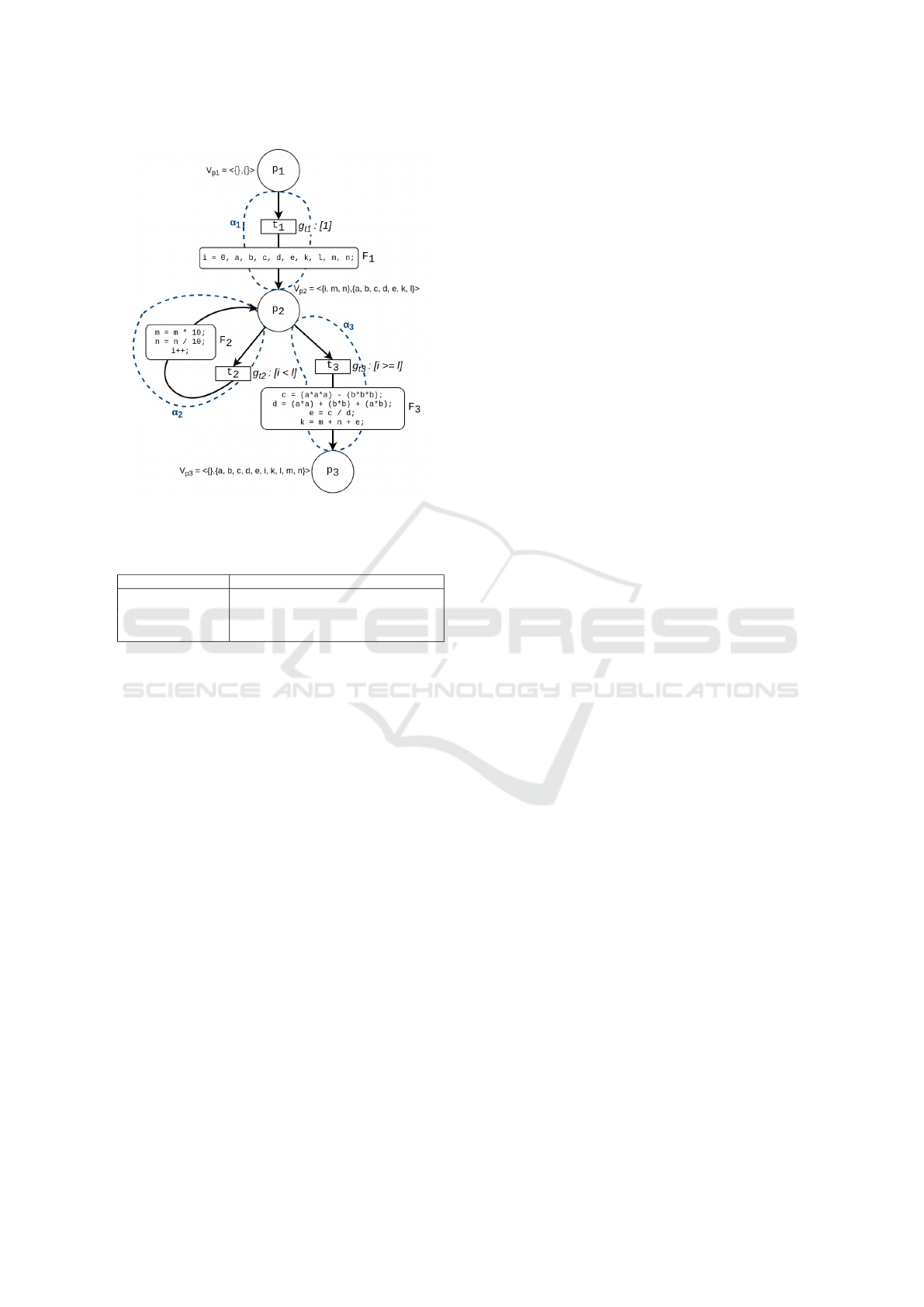
Figure 2: CPN model N

corresponding to the source pro-

gram in Listing 1.

Table 1: Informal transformation mapping.

Control Flow Graph Petri net

state place

transition in-coming arc, transition, out-going arc

transition condition guard condition associated with transition

transition function function-set associated with out-going arc

that are neither in-ports nor out-ports, there are two

kinds of such variables: changed variables and un-

changed variables. Changed variables are those vari-

ables whose values are changed from when the token

was last in the place. Similarly, unchanged variables

are those whose values don’t change. The partition

between changed and unchanged variables for each

place, is deﬁned dynamically during the computations

of the Petri net and the same will be illustrated in the

next subsection. Out-ports have no changed variables

in the associated variable vector.

3.2 Model Construction

Using compiler internal infrastructure, the program

can be transformed into an intermediate representa-

tion. This representation can be transformed to a Con-

trol Flow Graph (CFG) using the fdump process of the

GCC compiler. In Table 1, we present an informal

mapping from CFG to the proposed Petri net model.

3.3 Computation Methodology

Fig. 2 depicts the CPN model N

for the source pro-

gram in Listing 1. The program is initialized with a

token in place p

, which is the in-port. The transition

is now enabled and consequently ﬁred. For exam-

ple, the user inputs values a = 4, b = 2, l = 3, m = 1

and n = 7425. The token is removed from

◦

= {p

and moved to t

◦

= {p

}. The function-set F

con-

tains the arithmetic expressions that initialize the vari-

ables i, a, b, c, d, e, k, l, m, n. The variable vector is

an ordered pair, the ﬁrst element represents the set

of changed variables, and the second element repre-

sents the set of unchanged variables. When a place is

marked for the ﬁrst time, all associated variables are

considered as unchanged variables. The variable vec-

tor V

at this point is h{}, {a, b, c, d, e, i, k, l, m, n}i.

Now, the guard conditions of t

and t

are evalu-

ated. Since initially g

(i.e. i = 0 < l = 2) is true,

it is ﬁred and the token moves from p

back to p

but with values changed according to the expressions

in F

(now i = 1, m = 10, n = 742). Consequently,

since the values of i, m, n differ from their value as-

sociated previously with p

, they are considered as

changed variables. The variable vector is updated to

= h{i, m, n}, {a, b, c, d, e,k, l}i.

This cycle is repeatedly traversed until i = 3 (and

m = 1000, n = 7) and the guard condition g

ceases

to be true. This captures the while loop in the pro-

gram that calculates the values of m and n while in-

crementing the value of i. The termination of the

loop is captured by transition t

with the guard con-

dition i ≥ l. Now that t

is disabled and t

is en-

abled, t

is ﬁred, and the token is moved from p

to p

. The value vector of the token is changed ac-

cording to the expressions in F

. The variable vector

for p

, V

= h{}, {a, b, c, d, e, i, k, l, m, n}i This sig-

nals the termination of the program since no more

transitions are enabled. Finally, c = 56, d = 28, e = 2,

k = 1009

Fig. 3 depicts the CPN model N

for the trans-

lated program in Listing 2. As before, t

is ﬁred and

the token is removed from p

and added to p

and p

simultaneously. This is how the Petri net modelling

paradigm captures parallelism. At this point, the vari-

able vectors V

= V

= h{}, {i, j, a, b, e,k, l, m, n}i.

Now, g

, g

, and g

are simultaneously evaluated.

Since g

and g

are satisﬁed, transitions t

and t

are

both ﬁred simultaneously.

The value vectors in the tokens are updated ac-

cording to the respective associated functions-sets,

and sent back to the respective places. Since the val-

ues of i, m have changed for p

and j, n have changed

for p

, the variable vectors for these places are up-

dated as follows: V

= h{i, m}, { j, a, b, e, k, l, n}i

and V

= h{ j, n}, {i, a, b, c,d, e, k, m}i respectively.

These loops are traversed simultaneously until both

and g

are false.

ICSOFT 2021 - 16th International Conference on Software Technologies

536

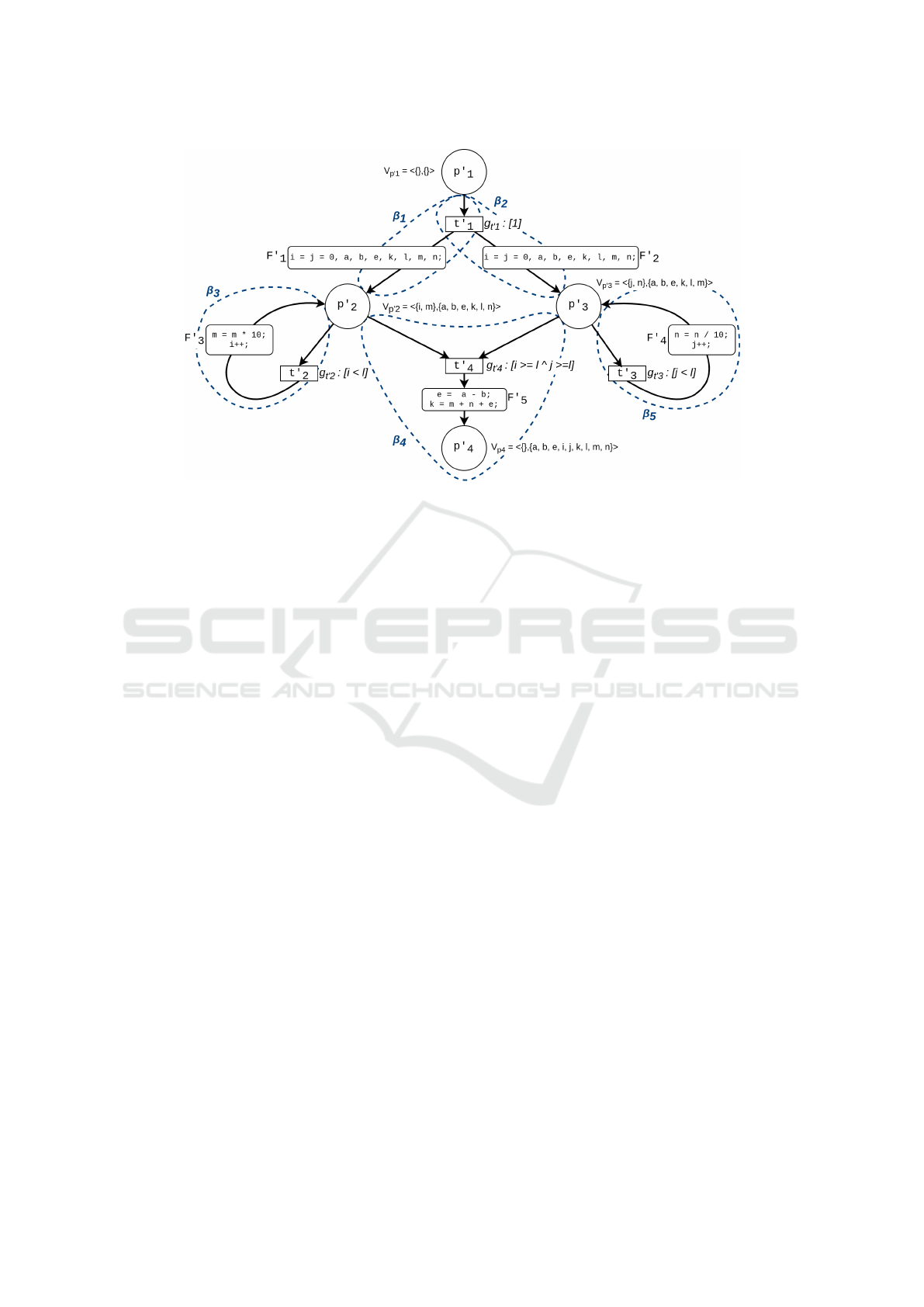
Figure 3: CPN model N

corresponding to program in Listing 2.

At this point, to evaluate g

, we have two sources of

values for the three variables i, j, l coming from the

tokens in p

and p

. In such cases of conﬂict, the vari-

able value from the place which has the variable as a

changed variable in its variable vector is given prece-

dence. That is, since i is a changed variable for p

, the

value for i is selected from p

. Similarly, the value of

j is selected from p

. In the case of l, since it is an un-

changed variable in both the places, its value in both

tokens is compared. If equal (which is the case), there

is no conﬂict; if unequal, an error is thrown. Since

is now enabled, it is ﬁred, and as before, p

, now

has the token with a value vector updated according

to the function-set F

. The values of the variables are

the same as that in the source Petri net N

A computation µ

out

in a Petri net is deﬁned as the

sequence of markings from in-port to out-port. So the

computations in the above examples can be written

mathematically as:

= h{p

}, {p

}

, {p

3.4 Notion of Path on CPN Model

In the previous section, we have seen a set of com-

putations involving loops. In a general program, the

number of loop traversals is unbounded. Therefore,

we cannot characterize the set of computations and

we cannot establish computational equivalence be-

tween two models. From the classical program veri-

ﬁcation techniques, we introduce the concept of ﬁnite

paths such that any computation can be represented in

terms of a ﬁnite set of paths. To construct the path, we

need to introduce the notion of cut-points. Using (at

least one) cut-points we ‘cut’ each loop to construct

a ﬁnite number of paths. The notion of cut-points in

our CPN model is as follows:

1. All in-ports, ∀p ∈ P

, are cut-points.

2. All out-ports, ∀p ∈ P

out

, are cut-points.

3. All places that have back-edges are cut-points.

A path is a sequence of out-going arcs from a set of

cut-points to a cut-point, while having no cut-point in

between. Through the backward cone of foci method,

we construct the paths in the Petri net model. The

detailed discussion of the path construction algorithm

is given in (Bandyopadhyay, 2016). It is to be noted

that if an out-going arc is covered in one path, it need

not be considered in another path.

From the above rules for cut-points, the set of cut-

points in the source model N

in Fig. 2 is {p

, p

Starting from p

, we obtain the path α

= h(t

, p

from p

to p

. Similarly, we obtain two more paths:

= h(t

, p

)i, from p

back to p

and α

= h(t

, p

from p

to p

In the translated model N

in Fig. 3 the set of

cut-points is {p

, p

}. Starting from p

, we

can construct two paths β

= h(t

, p

)i to p

and

= h(t

, p

)i to p

. Now, from p

, we obtain two

paths: β

= h(t

, p

)i which captures the loop from

back to p

and β

= h(t

, p

)i from p

and p

. Similarly, we obtain the path β

= h(t

, p

)i from

back to p

3.5 Validity of PBEC

To prove the validity of the path-based equivalence

checker, we show that any computation can be repre-

Towards an Approach for Translation Validation of Thread-level Parallelizing Transformations using Colored Petri Nets

537

sented as a concatenation of parallel paths.

As an example, taking the translated model N

Fig. 3, we can express the computation as follows:

= h{p

}, {p

, p

}

l+1

, {p

We can express the same computation in terms of the

sequence of transitions that are ﬁred. In order to do

so, the i

element of the computation in terms of the

transitions, is(are) the transition(s) that ﬁre(s) when

moving from the i

to i+ 1

marking. Following this

principle, we obtain the computations for the trans-

lated model as:

= h{t

}, {t

}

, {t

We can now express the computation in terms of the

out-going arcs. To do this, we can simply replace

each transition with its corresponding set of out-going

arc(s):

= h{(t

, p

), (t

, p

)}, {(t

, p

), (t

, p

)}

, {(t

, p

)}i

For any computation µ

out

of an out-port p

out

of a

CPN model N with path-cover π, there exists a reor-

ganized sequence µ

, of paths in π, such that µ

' µ

The set of paths of N

, π

= {β

, β

Initially, µ

= φ. The last member of µ

is (t

, p

The path β

has (t

, p

) as its last member. So β

is prepended to µ

, and all the out-going arcs in β

(only (t

, p

)) are removed once from µ

Now, the last member of µ

is {(t

, p

), (t

, p

)}.

, p

) is the last member of β

and (t

, p

) is the

last member of β

. So {β

||β

} is prepended to µ

and all the out-going arcs from β

and β

are removed

once from µ

. This step will be repeated l − 1 times

until the only element left in µ

is {(t

, p

), (t

, p

)}.

Since (t

, p

) is the last element of β

and (t

, p

) is

the last element of β

, {β

||β

} is prepended to µ

The algorithm is now terminated since µ

is empty.

Therefore

= h{β

||β

}, {β

||β

}

, {β

3.6 Equivalence Checking Mechanism

There are two entities associated with every path

1. Condition of Execution, R

, which is associated

with the guard conditions g

, of the transitions as-

sociated with the path.

2. Data Transformation, r

, which is associated with

the function-set F of the transitions associated

with the path.

Two paths α and β are considered equivalent when

' R

and r

= r

. The equivalence checking

mechanism is based on the principle: “∀ α ∈ π

∃ β ∈ π

and ∀ β ∈ π

, ∃ α ∈ π

| α ' β =⇒

' π

=⇒ N

' N

”. During checking, the al-

gorithm constructs correspondence relationships be-

tween the places, variables, and transitions, respec-

tively. To check two arithmetic or logical expres-

sions, we integrate the Z3 Theorem Prover with the

equivalence checker, to further extend the equivalence

checking capability. Following are the informal al-

gorithmic steps for checking equivalence between N

and N

In our motivating example, the set of paths in N

and N

are {α

, α

} and {β

, β

} re-

spectively. Also, R

= g

, R

= g

, R

= g

and

= F

, r

= F

, r

= F

. Similarly, R

= R

, R

= g

, R

= g

, R

= g

and r

= F

, r

= F

, r

= F

, r

= F

Step 1). Taking the ﬁrst element of π

, i.e. α

we look at its pre-place p

. Places p

and p

cor-

respond to each other since they are in-ports. Since

is a pre-place for paths β

and β

, these two paths

are candidate paths for α

. The SMT solver tells us

that R

' R

(i.e. g

= g

) and R

' R

(i.e.

= g

). The SMT solver also tells us that r

(i.e. F

= F

) and r

= r

(i.e. F

= F

). Hence,

' β

and α

' β

From this information we also infer that the post-

places of these paths correspond to each other, i.e. p

corresponds to p

and p

Step 2). Taking the next element of π

i.e. α

The pre-place of α

is p

, which corresponds to p

and p

. Since β

and β

have the two places respec-

tively as their pre-place, they are candidate paths for

. Checking for equivalence between these paths

results in a ‘No’ answer from the SMT solver. So,

we go for path merging. The paths β

and β

can

be merged parallelly, due to place, variable, and tran-

sition correspondence. The SMT solver tells us that

' R

kβ

. Similarly, r

= r

kβ

. Hence, α

(β

k β

Step 3). Finally, taking the path α

, it’s pre-place

is p

which has correspondence to p

and p

, which

are the pre-places of β

. Similarly, the post-place

of α

corresponds to the post-place of β

since they

are out-ports in their respective nets. Hence, β

is a

candidate path for α

. The SMT solver tells us that

' R

and r

= r

. Hence, α

' β

. So,

' β

,β

; α

' {β

k β

} ; α

' β

Since “∀ α ∈ π

∃ β ∈ π

| α ' β =⇒ π

' π

=⇒ N

' N

”. That is, the programs in Listing 1 and

Listing 2 are semantically equivalent.

ICSOFT 2021 - 16th International Conference on Software Technologies

538

In the following subsection, we brieﬂy describe

the Z3 Theorem Prover, it’s internal equivalence

checking mechanism, and how it will be integrated

with the path analyzer.

3.6.1 Z3 Theorem Prover

For two candidate paths α and β , the Z3 Theorem

Prover (Z3) receives the conditions of execution, R

and R

, and the data transformation, r

and r

, from

the path analyzer. All the program statements are en-

coded as Static Single Assignments to preserve the or-

der of execution. The sub-scripts ‘ s’ and ‘ t’ are ap-

pended for variables of P

and P

respectively. The

input to Z3 consists of:

1. Variables and corresponding type declarations.

2. Functions in the form of assert statements

3. Test statements asserted as negations. Z3 returns

a sat (true) answer if it ﬁnds even one case (from

the entire model space) that satisﬁes equivalence.

Using the negation, we can test that equality is

satisﬁed over the entire model space. Mathemat-

ically: for ξ (the model space) and c (the cases),

by De Morgan’s Law, ¬(

c∈ξ

c) =

c∈ξ

¬c.

So, an unsat output from Z3 actually corresponds to

equivalence and a sat output implies non-equivalence.

Also, the test statements check for equality only be-

tween the common variables of P

and P

. In case of

multiple assignment of the same variable, only the last

executed variable is considered (i.e. the variable with

highest numerical sufﬁx).

As an example, in Step 3) for checking equiva-

lence between the paths α

and β

, the Z3 input is as

follows:

1(declare- con s t g_t3_ s Bool )

2(declare- con s t g_t4_ t Bool )

3(declare- con s t i_0 _ s In t )

4(declare- con s t i_0 _ t In t )

5(declare- con s t j_0 _ t In t )

6(declare- con s t l_ s I nt )

7(declare- con s t l_ t I nt )

8(assert (= g _ t3_s ( >= i_0 _ s l_s )))

9(assert (= g _ t4_t ( and ( >= i_0 _ t l_ t )

10( >= j_0 _ t l_ t ))) )

11(assert (= l_s l_ t ))

12(assert (= i _0_s i _ 0_t ))

13(assert (= i _0_t j _ 0_t ))

14(assert (no t (= g _ t 3_s g_t 4 _ t )))

15(check- s at )

Listing 3: Checking equivalence of R

and R

In Listing 3, the ﬁrst two lines deﬁne the guard con-

ditions as Boolean functions. Lines 3-7 deﬁne the

associated variables. The next two lines 8-10 deﬁne

s = i ≥ l and g

t = i ≥ l & j ≥ l . To facilitate

equivalence checking, equivalence between variables

is asserted in lines 11-13. i 0 t = i 0 s is infered from

and F

. Next is the assert statement for equivalence

checking deﬁned as a negation. In the last statement

we check equivalence. Z3 returns unsat which im-

plies R

= R

. Similarly, to check the data transfor-

mation equivalence between the two paths, the corre-

sponding code is given in Listing 4.

1 (declare- c o nst a_s I nt )

2 (declare- c o nst a_t I nt )

3 (declare- c o nst b_s I nt )

4 (declare- c o nst b_t I nt )

5 (declare- c o nst c_s I nt )

6 (declare- c o nst d_s I nt )

7 (declare- c o nst e_s I nt )

8 (declare- c o nst e_t I nt )

9 (declare- c o nst k_s I nt )

10 (declare- c o nst k_t I nt )

11 (declare- c o nst m _1_ s In t )

12 (declare- c o nst m _1_ t In t )

13 (declare- c o nst n _1_ s In t )

14 (declare- c o nst n _1_ t In t )

15 (assert (= a_s a_ t ))

16 (assert (= b_s b_ t ))

17 (assert (= m_1 _s m _ 1_t ))

18 (assert (= n_1 _s n _ 1_t ))

19 (assert (= c_s ( -(* a_ s (* a _s a_ s ))

20 (* b_s (* b_s b_s )))) )

21 (assert (= d_s (+( * a _s a_ s ) ( +(* b_s b_s )

22 (* a_s b _s ) ) )))

23 (assert (= e_s ( div c _s d_ s )))

24 (assert (= k_s (+ m _ 1_s (+ n _1_s e_ s )) ))

25 (assert (= e_t (+ a_t b_t )))

26 (assert (= k_t (+ m _ 1_t (+ n _1_t e_ t )) ))

27 (assert ( n ot ( an d (= a_s a_ t )

28 ( and (= b_s b_t )

29 ( and (= m_1 _s m_ 1_t )

30 ( and (= e_s e_t )

31 ( and (= n_1 _s n_ 1_t )

32 (= k_s k _t )) ) ) ))))

33 (check- s at )

Listing 4: Checking equivalence of r

and r

In Listing 4, the lines 1-14 declare the associated vari-

ables. Lines 15-18 assert the equivalence for a, b, m, n

between the source and translated program. Lines 19-

24 serve as an assertion for the computations in F

and lines 25-26 assert the computations in F

. Finally,

lines 27-30 comprise the assertion statement in nega-

tion for equivalence checking between all the corre-

sponding deﬁned variables and the statement in line

31 checks for equivalence. Z3 gives the result unsat

for the check, which implies that r

= r

Towards an Approach for Translation Validation of Thread-level Parallelizing Transformations using Colored Petri Nets

539

Table 2: Model size for different Petri-net PBEC.

Example

ST-1 ST-2 Proposed

p t p t p t

BCM 34 28 6 6 3 2

MINMAX 31 27 7 7 4 6

PETERSON 11 9 4 2 6 8

DEKKERS 19 14 6 4 6 8

LUP 28 21 6 4 10 16

Table 3: Capabilities of different PBEC.

Example FSMD-VP FSMD-EVP ST-1 ST-2 Proposed

BCM X X X X X

MINMAX X X X X X

PETERSON X X X X X

DEKKERS X X X X X

LUP X X X X X

4 EXPERIMENTAL RESULTS

We have manually tested our equivalence checking

algorithm on ﬁve examples, where parallelising trans-

formations are applied using Pluto (Bondhugula et al.,

2008) and Par4All (Amini et al., 2012) compilers.

BCM is a toy code for validating Basic Code Motion

technique, where some polynomial arithmetic oper-

ations are applied in the basic blocks. PETERSON

and DEKKERS are implementations of classical so-

lutions to the mutual exclusion problem of two con-

current processes. In the critical section, some poly-

nomial expression computation is present. LUP com-

putes the LU-decomposition with Pivoting, for a ma-

trix. We have only taken the pivoting routine which

does not contain any array. The details for LUP are

given in the PLuTo example suite (Bondhugula et al.,

2008). MINMAX computes the sum of the maximum

of four numbers (n

, n

) and the minimum of

four numbers (n

, n

). The programs and their

descriptions can be found in (Bandyopadhyay, 2016).

Table 2 presents a comparative study of the model

size of our proposed approach with the models of two

other Petri net-based equivalence checking tools ST-1

(Bandyopadhyay et al., 2017) and ST-2 (Mittal et al.,

2020). It is to be noted that the model size of the

current method is comparable with ST-2.

Table 3, presents several parallelizing and arith-

metic transformation veriﬁcation capabilities of the

proposed approach, compared with ST-1, ST-2 and

two CDFG (Control Data Flow Graph) based PBEC

namely, FSMD-VP (Finite State Machine with Datap-

ath and Value Propagation) (Banerjee et al., 2014) and

FSMD-EVP (Finite State Machine with Datapath and

Extended Value Propagation) (Chouksey et al., 2019).

It is to be noted that both FSMD based PBEC can-

not handle the parallelizing transformations because

FSMD is a sequential model of computation. ST-1

and ST-2 cannot handle arithmetic transformations.

They have their own normalizer, which affects their

limitations. These limitations are overcome by Z3.

5 RELATED WORK

Translation validation was introduced in (Pnueli et al.,

1998) and was demonstrated in (Necula, 2000) and

(Rinard and Diniz, 1999). The approach was further

enhanced in (Kundu et al., 2008) where they veri-

ﬁed the high-level synthesis tool named SPARK. All

these techniques are bisimulation based methods. A

loop parallelizing transformation validation method

comprising rewrite rules has been reported in (Bell,

2013). A bisimulation method for parallel programs

is also reported in (Milner, 1989). Another equiv-

alence checking method is the inductive-inferencing

based technique reported in (Felsing et al., 2014). The

method only works for scalar handing programs. It

compares the coupling predicates between two pro-

grams.

A major limitation of these methods is that the ter-

mination is not guaranteed. To alleviate this short-

coming, a path based equivalence checker for the

FSMD model was proposed for uniform and non-

uniform code motions, code motion across loop and

loop invariant code optimizations in (Karfa et al.,

2012; Banerjee et al., 2014; Chouksey et al., 2019).

However, these methods cannot handle loop swapping

transformations and many thread-level parallelizing

transformations because FSMDs cannot capture par-

allel behaviors easily.

The literature records no signiﬁcant attempts for

devising formal equivalence checking methods using

Petri net based models which is essentially a paral-

lel model of computationm; although, there are sev-

eral works on property veriﬁcation using Petri net

modelling paradigm (Lime et al., 2009; Charron-Bost

et al., 2013; Corradini et al., 2013; Westergaard,

2012). In (Bandyopadhyay et al., 2018), the valida-

tion of loop swapping and thread level parallelising

transformations using Petri net based models of pro-

grams was reported. However, the model size of the

method is not tractable. The major limitation of this

method is it cannot handle loop invariant code motion

as well as polynomial arithmetic transformations. To

overcome the limitations, a modiﬁcation in the model

construction as well as equivalence checking was re-

ported in (Mittal et al., 2020). However, the method

cannot handle polynomial arithmetic transformations.

ICSOFT 2021 - 16th International Conference on Software Technologies

540

6 CONCLUSION

In this paper we presented our ongoing work on devel-

oping an approach to check the equivalence of soft-

ware programs using a novel translation validation

technique for handling loops. In addition, our ap-

proach makes use of SMT solvers to validate arith-

metic transformations. Such constructions cannot be

handled by state-of-the-art equivalence checkers.

We presented an initial validation of the approach

for a standard benchmark. Currently this valida-

tion was performed manually. Therefore, our future

work is to implement a tool-chain supporting the ap-

proach and validate it on a larger benchmark. For

this, we will reuse existing compiler front-ends (e.g.

GCC) and automatically construct the Petri Net mod-

els from the generated intermediate code representa-

tion so that the approach can be tested on different

programming languages, potentially including exist-

ing architecture description languages such as UML,

SysML and AADL. This will also allow us to fur-

ther characterize the domain of applicability of the ap-

proach; i.e. which language constructions and trans-

lations are handled by our approach and to evaluate

scalability for large programs.

ACKNOWLEDGEMENT

The authors would like to thank Didier Buchs and

Dipankar Sarkar for initial ideas regarding the reﬁne-

ment of the Petri net model.

REFERENCES

Amini, M., Creusillet, B., Even, S., Keryell, R., Goubier,

O., Guelton, S., Mcmahon, J., Pasquier, F.-X., P

ean,

G., and Villalon, P. (2012). Par4all: From convex ar-

ray regions to heterogeneous computing. Workshop

IMPACT.

Bacon, D. F., Graham, S. L., and Sharp, O. J. (1994). Com-

piler transformations for high-performance comput-

ing. ACM Computing Survey, 26(4).

Bandyopadhyay, S. (2016). Path based equivalence check-

ing of Petri net representation of programs for trans-

lation validation. PhD thesis, IIT, Kharagpur.

Bandyopadhyay, S., Sarkar, D., and Mandal, C. (2018).

Equivalence checking of petri net models of programs

using static and dynamic cut-points. Acta Informatica.

Bandyopadhyay, S., Sarkar, S., Sarkar, D., and Mandal,

C. A. (2017). Samatulyata: An efﬁcient path based

equivalence checking tool. In ATVA.

Banerjee, K., Karfa, C., Sarkar, D., and Mandal, C. (2014).

Veriﬁcation of code motion techniques using value

propagation. IEEE TCAD, 33(8).

Banerjee, K., Sarkar, D., and Mandal, C. (2014). Extend-

ing the fsmd framework for validating code motions

of array-handling programs. IEEE TCAD, 33(12).

Bell, C. J. (2013). Certiﬁably sound parallelizing transfor-

mations. In CPP, pages 227–242.

Bondhugula, U., Hartono, A., Ramanujam, J., and Sadayap-

pan, P. (2008). Pluto: A practical and fully automatic

polyhedral program optimization system. In PLDI.

Charron-Bost, B., Merz, S., Rybalchenko, A., and Wid-

der, J. (2013). Formal veriﬁcation of distributed algo-

rithms (dagstuhl seminar 13141). Dagstuhl Reports,

3(4):1–16.

Chouksey, R., Karfa, C., and Bhaduri, P. (2019). Translation

validation of code motion transformations involving

loops. IEEE TCADICS, 38(7).

Corradini, A., Ribeiro, L., Dotti, F. L., and Mendizabal,

O. M. (2013). A formal model for the deferred up-

date replication technique. In TGC.

de Moura, L. and Bjørner, N. (2008). Z3: An efﬁcient smt

solver. In TACAS, pages 337–340.

Felsing, D., Grebing, S., Klebanov, V., R

ummer, P., and Ul-

brich, M. (2014). Automating regression veriﬁcation.

In ACM/IEEE International Conference on ASE.

Jensen, K. and Kristensen, L. M. (2009). Coloured Petri

Nets - Modelling and Validation of Concurrent Sys-

tems. Springer.

Karfa, C., Mandal, C., and Sarkar, D. (2012). Formal ver-

iﬁcation of code motion techniques using data-ﬂow-

driven equivalence checking. ACM TODAES, 17(3).

Kundu, S., Lerner, S., and Gupta, R. (2008). Validating

high-level synthesis. CAV.

Lime, D., Roux, O. H., Seidner, C., and Traonouez, L.

(2009). Romeo: A parametric model-checker for petri

nets with stopwatches. In TACAS.

Milner, R. (1989). Communication and Concurrency.

Prentice-Hall, Inc.

Mittal, R., Banerjee, R., Sarkar, S., and Bandyopadhyay, S.

(2020). Translation validation of loop involving code

optimizing transformations using petri net based mod-

els of programs. In PNSE Workshop.

Necula, G. C. (2000). Translation validation for an optimiz-

ing compiler. In PLDI.

Pnueli, A., Siegel, M., and Singerman, E. (1998). Transla-

tion validation. In TACAS.

Rinard, M. and Diniz, P. (1999). Credible compilation.

Technical Report MIT-LCS-TR-776, MIT.

Westergaard, M. (2012). Verifying parallel algorithms and

programs using coloured petri nets. Trans. on Petri

Nets and Other Models of Concurrency.

Towards an Approach for Translation Validation of Thread-level Parallelizing Transformations using Colored Petri Nets

541