Modelling Renewable Energy Sources for Harmonic Assessments in

DIgSILENT PowerFactory: Comparison of Different Approaches

Zhida Deng

, Grazia Todeschini

, Kah Leong Koo

and Maxwell Mulimakwenda

Faculty of Science and Engineering, Swansea University, Swansea, U.K.

Power Quality and Modelling Department, National Grid, Warwick, U.K.

Keywords: Harmonics, Power Quality, Power Systems Modelling, Renewable Energy Sources, Total Harmonic

Distortion, Voltage Unbalance.

Abstract: With the increasing number of Renewable Energy Sources connected to the power grid, the impact on system

operation is becoming more evident. To assess this impact, accurate computer models are required for both

the power system and the devices connected to it. Various types of system integration studies need to be

performed in order to study both steady-state and abnormal operation. Among the steady-state analyses, power

quality studies assess the impact of Renewable Energy Sources on parameters such as voltage levels and

harmonic content. Harmonic studies are gaining more attention because of the nature of renewable energy

sources which are mainly connected to the power grid through electronic power converters, thus producing

undesirable harmonics. This paper analyses various settings, solvers and harmonic source models in a

commercial software – DIgSILENT PowerFactory – to ensure accurate calculation and correct interpretation

of harmonic assessment. A simple model comprising seven harmonic devices is used for the analysis of

various case studies. Their results are then compared with the standard IEC model and recommendations are

proposed on how to appropriately model the RESs depending on the specific application considered.

1 INTRODUCTION

Existing power systems were designed decades ago

when fossil fuels (e.g. coal, gas, oil) were exclusively

employed to generate electricity. With growing

population and industrial expansion, has led to

increasing demands on power systems pushing them

closer to their operational limits. Challenges to reduce

greenhouse gases from conventional power stations

to tackle climate change have also raised more serious

concerns on the sustainability of fossil fuel-based

power generation. These concerns have fueled the

development of Renewable Energy Sources (RESs)

to meet future electricity demands and displace

conventional generations. It is expected that RESs

will make up to approximately 63.15% of total

installed generation capacity by 2050 in the UK,

according to the National Grid Future Energy

Scenarios report (National Grid ESO, 2019).

https://orcid.org/0000-0002-8448-1934

https://orcid.org/0000-0001-9411-0726

https://orcid.org/0000-0002-9549-8627

https://orcid.org/0000-0001-9433-4607

Since conventional power systems have not been

designed to operate not only with large number of

RES devices but also of increasing capacities, power

quality issues need to be managed to an acceptable

level. Increasing harmonic levels is identified as one

of the main areas of concern in relation to RESs

integration, and needs to be well studied and properly

managed, as reported in (Working Group JWG-

C4/C6.29, 2016). The voltage and current are

sinusoidal waveforms in an ideal Alternating Current

(AC) power system but are distorted by harmonics

that are produced by nonlinear loads and power

electronic-based devices, for example motor drives

and RES inverter (IEEE Power and Energy Society,

2014). These devices produce harmonics at multiple

or sub-multiple integers of fundamental frequency.

Small levels of harmonics are tolerated by equipment

and various standards have been developed for

harmonic control and to manage their connection to

the network (Energy Networks Association, 2020;

130

Deng, Z., Todeschini, G., Koo, K. and Mulimakwenda, M.

Modelling Renewable Energy Sources for Harmonic Assessments in DIgSILENT PowerFactory: Comparison of Different Approaches.

DOI: 10.5220/0010580101300140

In Proceedings of the 11th International Conference on Simulation and Modeling Methodologies, Technologies and Applications (SIMULTECH 2021), pages 130-140

ISBN: 978-989-758-528-9

IEC TR 61000-3-6, 2008; IEEE Power and Energy

Society, 2014). This is because excessive harmonic

levels may lead to various detrimental effects,

including dielectric failure, overheating of electrical

equipment, and false operation of circuit breakers

(Cherian et al., 2016). Since RESs are mainly based

on the use of power electronics, they inject harmonics

into the network. With rapidly increasing number of

these devices, even if individual units are compliant

with the standards, the combined effect of numerous

RESs installed in close proximity will lead to an

overall increase of harmonic levels in the system

(Koo & Emin, 2016).

Computer simulations are used to assess the

impact of RESs on harmonic levels on the network.

Both time-domain and frequency-domain methods

are used (Medina et al., 2013). Time-domain methods

characterise system behaviour using differential

equations, and individual harmonic components can

be derived via Fourier transformation. Although these

methods provide detailed and accurate models of non-

linear devices and their control algorithms, they do

not allow easy calculation of the system impedances

as well as modelling of the frequency-dependent

parameters (Medina et al., 2013).

Frequency-domain analysis methods, including

frequency scans, harmonic penetration studies and

harmonic load flows, are widely employed in

engineering practices to predict expected harmonic

distortions on the network. By performing frequency-

domain analysis, harmonic current and voltage

distortions on the network as well as resonances are

calculated. This process allows assessing compliance

with the standards and, if required, informs on

requirements for the filter design (Working Group

JWC-C4/B4.38, 2019). A frequency scan consists of

calculation of network impedance at various

frequencies to determine frequency responses of

power system and identify potential resonance

conditions; a harmonic penetration study refers to

nodal analysis for each harmonic order assuming no

interaction between fundamental and harmonic

components; a harmonic load flow uses Newton-

Raphson or Gauss-Seidel based algorithm to solve

unified fundamental and harmonic power flow

equations, as described in (Herraiz et al., 2003;

Medina et al., 2013). It is important to observe that in

practice, the terms ‘harmonic load flow’ and

‘harmonic penetration studies’ are often used

interchangeably, but these approaches may produce

different results. Hence, it is important to understand

the assumptions underlying the software and the

solver under consideration.

Frequency-domain analysis can be carried out for

balanced and unbalanced systems. In practical power

systems, unbalance between phases is small from

asymmetry in transmission systems and the nature of

the loads and generating sources are normally

unbalanced, therefore a balanced frequency-domain

analysis is generally sufficient. However, unbalanced

harmonic analysis provides more accurate results

when studying asymmetrical systems, either in terms

of network configuration (Jensen, 2018), and/or

loads. In power systems where RESs are single-phase

connected, it may be necessary to consider unbalance

harmonic distribution between the phases in order to

carry out a more accurate assessment.

In addition to unbalance, the summation of

harmonics due to different sources and harmonic

source modelling is an important factor that will also

has an impact on the accuracy of the results. For

harmonic summation, two approaches are mainly

used: (1) either the magnitude and phase are

considered for each harmonic component, (2) or the

summation rule described in standard IEC 61000-3-6

(IEC TR 61000-3-6, 2008) is employed. In the latter

case, a summation exponent is considered to take into

account harmonic phase angles at higher harmonic

orders. While IEC summation rule is based on

practical considerations, it may result in inaccurate

assessment of harmonic level at the Point of Common

Coupling (PCC) (Eltouki et al., 2018; Working Group

JWG-C4/C6.29, 2016) – i.e. at the point where

multiple loads or sources connect to the system. This

discrepancy may be due to the harmonic components

adding or cancelling to varying degrees due to the

harmonic phase angle differences, where this

phenomenon may not be taken into account

accurately when applying the IEC summation rule.

As in (Ghassemi & Koo, 2010), different modelling

approaches are described to calculate the harmonic

distortion at the PCC for an offshore wind farm, and

the limitations of the IEC summation rule are

highlighted.

With large penetration of power converters, such

as the ones used for RESs, it is more likely that

harmonic phase angles will be randomly varying

within a reasonable range (Bećirović et al., 2018).

Under these conditions, it is more appropriate to carry

out harmonic analysis by varying the harmonic phase

angles to provide a more realistic harmonic

assessment. Although the topic of harmonic

assessment for RESs is not new, not many research

works can be found considering the impact of IEC

summation rule, appropriate use of harmonic models,

and system unbalance conditions at the same time.

Modelling Renewable Energy Sources for Harmonic Assessments in DIgSILENT PowerFactory: Comparison of Different Approaches

131

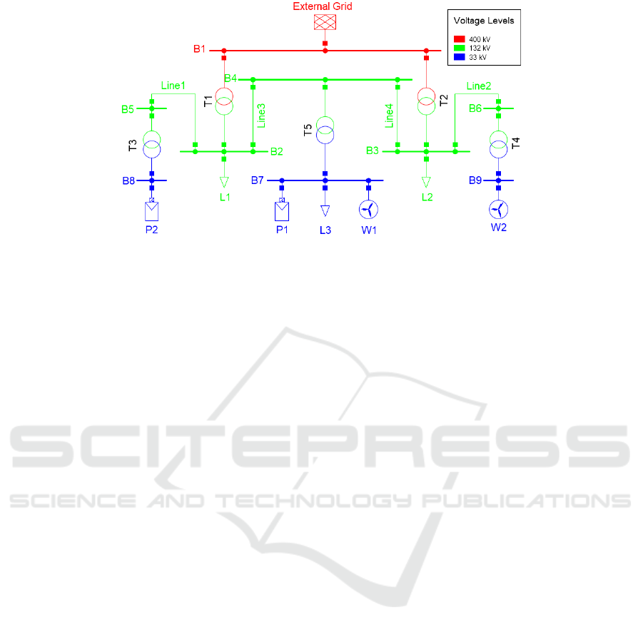
Figure 1: Single-line diagram of the simulated network.

The commercial software – DIgSILENT

PowerFactory (DPF) (DIgSILENT, 2020a) – is

widely used to perform power quality assessments

and provides numerous options to carry out harmonic

analysis. These options include: harmonic source

models (named IEC source and Unbalance Phase

Correct source), summation rules and solvers. If these

options are not used appropriately to model the actual

equipment, results may vary significantly, thus

leading to misleading harmonic assessments.

Although the user manual (DIgSILENT, 2020b)

briefly explains the differences between these

options, it is not clear enough to understand their

impact on the harmonic assessment.

This work aims at examining the appropriate use

of different harmonic source models and choice of

harmonic load flow solvers available within DPF to

calculate harmonic levels in distribution and

transmission systems. This paper provides a better

understanding of using different options in DPF and

modelling guidance for unbalanced harmonic current

sources in a way that allows flexibility while at the

same time providing comparable results as the ones

provided by the IEC model. DPF is used here as it is

a widely used software in the power industry and

similar concerns may arise with other software.

A simple 9-bus network with 7 harmonic sources

is considered: the network is symmetrical in nature,

and unbalance is caused by the harmonic sources

only. Future work will address unbalanced networks.

In Section 2, the network and harmonic source

models are described. In Section 3, three test cases

with different number of harmonic sources are set up

for harmonic analysis. The frequency scans and

voltage Total Harmonic Distortions (THDs) obtained

from different solvers and harmonic source models

are compared and discussed. Finally, the possibility

of matching IEC harmonic current source model

using equivalent Unbalanced Phase Correct (UPC)

model is investigated.

2 SIMULATION NETWORK AND

HARMONIC SOURCE

2.1 Network Description

A 50 Hz symmetrical three-phase 9-bus network –

including 4 transmission lines, two photovoltaics

(PV) plants, 2 Wind Turbine Generator (WTGs), 3

Loads and 5 two-winding Wye grounded-delta (Yg-

d) connected transformers with 30-degree phase shift

was built in DPF, as shown in Figure 1. To ensure

convergence of the power flow at fundamental

frequency, an external grid element acting as slack

bus was used. Distributed-parameter line model was

adopted to consider the long-line effects (i.e. higher

frequencies increase the electrical distance of the line

(Working Group JWC-C4/B4.38, 2019)) during the

harmonic analysis. The voltage levels are indicated

by different colours, and the system component

specifications and power flow parameters are given in

Table 1.

2.2 Harmonic Source Modelling

In this paper, two constant harmonic current source

models available in DPF – UPC and IEC – were

considered. Harmonic current amplitudes (referred to

the fundamental current) up to the 50

harmonic

order found from the literature for loads (Preda et al.,

2012; Robinson, 2003), PV farms (Elkholy, 2019;

Erik & Leigh, 2016; Oliver et al., 2018; Rampinelli et

SIMULTECH 2021 - 11th International Conference on Simulation and Modeling Methodologies, Technologies and Applications

132

Table 1: System component parameters.

L1 L2 L3 P1 P2 W1 W2

𝑆



(

MVA

)

20 30 100 12 21 60 30

𝑃

(MW)

19 28.5 90 8 18 40 20

𝑄

(

Mvar

)

6.25 9.37 43.59 0 0 0 0

T1 – T2 T3 – T5

Voltage 400/132 kV 132/33 kV

𝑆



(MVA)

255 90

16% short-circuit

voltage with 1.8 MW

losses

13% short circuit

voltage with 0.25

MW losses

Line1 Line2 Line3 Line4

𝐿

(km)

15 20 24 31

𝑍

(Ω/km)

positive/negative-sequence R and X: 0.0212

and 0.1162;

zero-sequence R and X: 0.0848 and 0.4650

External Grid

Short-circuit power: 10000 MVA;

short circuit current: 14.43 kA; c-factor: 1.1;

R/X ratio: 0.1, R: 1.75 Ω, X: 17.51 Ω

Note that the symbols 𝑆



, 𝑃, 𝑄, 𝑍, 𝑅, 𝑋 and 𝐿 denote rated power,

active power, reactive power, impedance resistance, reactance, and

line length, respectively.

al., 2015) and wind farms (Ambrož et al., 2017;

Energyiforsk, 2018; Mendonça et al., 2012; Preciado

et al., 2015; Rauma, 2012) are given in Table 2. The

harmonic data for WTG at 42-50 orders is reported as

smaller than 0.1 in (Ambrož et al., 2017): without

loss of generality, the value of 0.1 was used in this

paper.

Since the harmonic current injection for the IEC

harmonic model in DPF can only be based on the

rated current, the rated current (𝐼



) was chosen as the

reference current for the UPC model to ensure the

same amount of harmonic current injections as the

IEC model. For modelling the IEC harmonic current

source, the data given in Table 2 were used as

harmonic current injections and the standard IEC or

self-defined summation rule can be selected to take

into account the harmonic phase angles. The standard

IEC summation rule is expressed as (IEC TR 61000-

3-6, 2008):

𝐼





∑

𝐼















(1)

𝛼=

1 i

ℎ<5

1.4 i

5≤ℎ≤10

2 i

ℎ>10

(2)

Table 2: Harmonic current injection data.

ℎ

Load

𝐼



/𝐼



(%)

𝐼



/𝐼



(%)

WTG

𝐼



/𝐼



(%)

ℎ

Load

𝐼



/𝐼



(%)

𝐼



/𝐼



(%)

WTG

𝐼



/𝐼



(%)

1 100 100 100 26 - 0.04 0.02

- 0.11 0.10

- 0.02 0.02

0.15 0.15 0.10

- 0.08 0.02

- 0.10 0.10

0.11 0.05 0.03

0.37 0.16 0.40

- 0.05 0.01

- 0.03 0.14

- 0.11 0.02

0.28 0.18 0.07

- 0.05 0.01

- 0.04 0.06

- 0.02 0.02

0.27 0.04 0.05

0.09 0.03 0.02

- 0.04 0.04

0.09 0.03 0.04

0.41 0.12 0.06

- 0.00 0.04

- 0.01 0.03

- 0.02 0.04

0.12 0.11 0.05

- 0.01 0.06

- 0.03 0.02

- 0.08 0.06

- 0.02 0.02

- 0.10 0.06

- 0.02 0.01

- 0.13 0.05

0.16 0.06 0.03

- 0.02 0.10

- 0.04 0.01

- 0.08 0.10

0.08 0.05 0.03

- 0.08 0.10

- 0.02 0.01

- 0.10 0.10

0.08 0.02 0.01

- 0.02 0.10

- 0.02 0.01

- 0.11 0.10

0.60 0.07 0.02

- 0.10 0.10

- 0.01 0.01

- 0.13 0.10

0.08 0.09 0.02

- 0.01 0.10

Notation ‘ℎ’ denotes the harmonic order, ‘𝐼



’ and ‘𝐼



’ refer to

harmonic current at order ℎ and reference current, respectively.

where 𝐼



is the harmonic current at ℎ



harmonic

order, 𝑁 is the number devices connected at PCC and

𝛼 is the summation exponents for different harmonic

orders.

For modelling the UPC current harmonic sources,

the harmonic current amplitudes of three phases were

set to be identical to allow comparisons with the IEC

model. The actual three-phase harmonic phase angles

of the UPC model are calculated as 𝜑





=∆𝜑





ℎ𝜑





, 𝜑





=∆𝜑





+ℎ𝜑





and 𝜑





=∆𝜑





+ℎ𝜑





(DIgSILENT, 2020b), where ℎ is the harmonic order,

and 𝜑





, 𝜑





and 𝜑





are the fundament current angles

of phase A, B and C, respectively. The phase

parameters ∆𝜑





, ∆𝜑





and ∆𝜑





used to specify each

harmonic phase angle were set to 0 for positive (e.g.

4, 7, 10, …) and negative-sequence (e.g. 2, 5, 8, …)

orders. Since the triplen harmonics in IEC source are

considered as positive-sequence, the ∆𝜑





, ∆𝜑





and

∆𝜑





in UPC model were set to 0, -120 and 120,

respectively to enable modelling of zero-sequence

components (i.e. triplen harmonics) to be considered

as positive-sequence as in the IEC model. Therefore,

the UPC harmonic source is effectively modelled as a

balanced harmonic model, similar to the IEC

Modelling Renewable Energy Sources for Harmonic Assessments in DIgSILENT PowerFactory: Comparison of Different Approaches

133

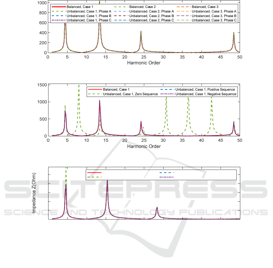
Figure 2: Balanced and unbalanced impedance characteristics at B2 for Case 1, Case 3 and Case 3.

Figure 3: Balanced and unbalanced impedance characteristics at B2 of Case 1.

Figure 4: Balanced and unbalanced impedance characteristics at B2 of Case 1 under ideal system conditions.

harmonic source, so that the results from the two

models can be compared.

3 SIMULATION RESULTS AND

DISCUSSION

This section first presents impedance characteristics

obtained from balanced and unbalanced frequency

sweep analysis when IEC and UPC model are used.

Then, various harmonic load flow calculations are

performed using different solvers, to compare the

voltage THD values and examine the differences

between the IEC and the UPC model. Finally, the

possibility of matching the IEC model using an

equivalent UPC model is studied and discussed.

3.1 Frequency Scan Analysis

The frequency scan analysis can be seen as solving

the network equation 𝑰



=𝒀



𝑽



(Medina et al.,

2013). where 𝑰



, 𝑽



and 𝒀



are current vector,

voltage vector and admittance matrix at harmonic

order ℎ, respectively. Injecting one pu current and

calculating the corresponding voltage, the system

admittance is obtained. Under the assumption of

system linearity, the frequency scan analysis always

produces the same impedance characteristics

regardless harmonic injection values, the type of

harmonic source model and the number of harmonic

sources. The approach described above is used by

DPF and other commercial software to calculate the

system impedance. In order to verify this assumption,

the balanced and unbalanced frequency scans were

Impedance Z(Ohm)

0 5 10 15 20 25 30 35 40 45 50

Harmonic Order

200

400

600

800

1000

Balanced, Case 1

Unbalanced, Case 1, Zero Sequence

Unbalanced, Case 1, Positive Sequence

Unbalanced, Case 1, Negative Sequence

SIMULTECH 2021 - 11th International Conference on Simulation and Modeling Methodologies, Technologies and Applications

134

calculating by injecting 10 Hz step size harmonic

current up to 2.5 kHz, under following cases:

• Case 1: IEC model adopted for 3 loads, 2 PVs

and 2 WTGs.

• Case 2: UPC model adopted for the 3 loads, 2

PVs and 2 WTGs.

• Case 3: no harmonic source model is

considered.

The impedance characteristics at the 132 kV

busbar B2 for the different cases are presented in

Figure 2. The frequency response at B2 for the tested

cases was exactly the same no matter the type and

number of harmonic sources, and the selection of

balanced or unbalanced frequency scan. These

findings were also verified to other busbars.

In addition to above tests, the impedance

characteristics between balanced and unbalanced

components are compared, as shown in Figure 3.

Although Figure 3 only shows the frequency

characteristics of Case 1, the same results were found

for Case 2 and 3. It can be seen that the balanced,

unbalanced positive-sequence and negative-sequence

share the same impedance characteristics, and their

resonance frequencies occur at the 4

, 13

, 24

and

orders. This is because the balanced frequency

scan in DPF considers the positive-sequence

component only. The resonance frequency of

unbalanced zero-sequence shown additional resonant

frequencies at the 8

, 31

, 37

and 43

orders. These

results are expected – the resonances of zero-

sequence are shifted when performing unbalanced

frequency scan, mostly due to the Yg-d connection of

the transformers and the difference between and zero

and positive/negative-sequence impedances of the

network components. Based on these considerations,

balanced and unbalanced frequency scans were

performed under an ideal system conditions, where

Yg-Yg connection was used, and positive/negative

and zero-sequence impedances of the transmission

lines and transformers were set to equal, with results

shown in Figure 4. In this case the resonance

frequencies (i.e. 5

, 15

, and 28

harmonic orders) of

balanced and unbalanced components are identical.

The same behaviour was observed for Case 2 and

Case 3. It is therefore concluded that the network

parameters are the only factors influencing the

frequency scans.

3.2 Harmonic Load Flow Analysis

As reviewed in (Herraiz et al., 2003), different

harmonic load flow techniques may produce distinct

results. Therefore, it is necessary to understand which

technique is applied by each software in order to carry

out a correct assessment. For the specific case of DPF,

review of the manual (DIgSILENT, 2020b) and

discussion with the technical support led to conclude

that

the load flow solution is calculated at

fundamental frequency only, and a harmonic

penetration study is carried out by applying nodal

analysis at various harmonic orders. Although a ‘true’

harmonic load flow could provide more accurate

results by taking into account the voltage-dependent

nature of the system components, it requires

significant computational effort due to the process of

solving a large number of fundamental and harmonic

power flow equations simultaneously (Medina et al.,

2013). This may be the reason why harmonic

penetration is widely used in the great majority of

commercial software (Working Group JWC-

C4/B4.38, 2019).

The following three cases were considered to

compare the results of harmonic load flow analysis

using the IEC and the UPC model, based on the

selection of different harmonic load flow solvers

available in DPF:

• Case 4: balanced harmonic load flow,

considering positive- or negative-sequence

equivalent single-phase according to default

settings (positive-sequence impedance for

zero- and positive-sequence harmonic orders,

and negative-sequence impedance for

negative-sequence harmonic orders).

• Case 5: balanced harmonic load flow with

positive-sequence only (using positive-

sequence impedance for all harmonic orders).

• Case 6: unbalanced harmonic load flow that

considers positive or negative-sequence three-

phase components at the related harmonic

order.

When any IEC harmonic source model exists in the

DPF model, the harmonic currents or voltages are

processed using the selected harmonic summation

rule (i.e. with standard or self-defined summation

exponents).

3.2.1 Single Harmonic Source Test

In this test, the photovoltaic plant (P1) connected to

the 33 kV busbar B7 was the only harmonic

producing device in the network. This is a simple way

to verify the differences between IEC and UPC model

when different solvers are used. In Table 3, the

voltage THD values at different busbars for Case 4, 5

Modelling Renewable Energy Sources for Harmonic Assessments in DIgSILENT PowerFactory: Comparison of Different Approaches

135

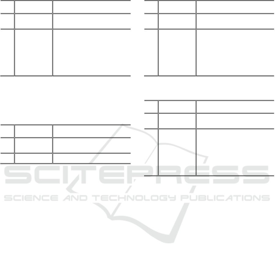
Table 3: Comparison of THDs between IEC and UPC

models under different cases (single harmonic source).

Standard IEC

model

UPC model

Bus

Case

4&5

(%)

Case 6

3-Ph

(

)

Case

4&5

(%)

Case 6

Ph-A

(%)

Case 6

Ph-B

(%)

Case 6

Ph-C

(%)

0.007 0.007 0.006 0.007 0.007 0.007

0.025 0.025 0.023 0.025 0.025 0.025

0.031 0.031 0.027 0.031 0.031 0.031

0.029 0.029 0.026 0.029 0.029 0.029

0.035 0.035 0.030 0.035 0.035 0.035

0.036 0.036 0.032 0.036 0.036 0.036

0.283 0.301 0.241 0.297 0.307 0.292

0.035 0.037 0.030 0.035 0.038 0.037

0.036 0.036 0.032 0.036 0.036 0.036

Bold values are all the same. ‘Ph-A’, ‘Ph-B’, ‘Ph-C’, and ‘3-Phase’

refer to phase A, phase B and phase C and all three phases,

respectively.

Table 4: THDs for IEC and UPC models at low-voltage

busbars under different cases when using Yg-yg

transformers (single harmonic source).

Standard IEC

model

UPC model

Bus

Case

4&5

(%)

Case 6

3-Ph

(

)

Case

4&5

(%)

Case 6

Ph-A

(%)

Case 6

Ph-B

(%)

Case 6

Ph-C

(%)

B7 0.283 0.283 0.241 0.283 0.283 0.283

0.035

0.035 0.030 0.035 0.035 0.035

and 6 are obtained, and the following conclusions can

be carried out:

• For the standard IEC model, all results are the

same for Case 4, 5 and 6 (three phases), except the

low-voltage busbar B7 and B8, because the use of

Yg-d connection at the 132/33 kV transformers

results in slightly different solutions of the

fundamental load flow for Case 6. By changing

the 132/33 kV transformers to Wye grounded-

wye grounded (Yg-yg) connection, the THDs at

B7 and B8 are the same (bold values in Table 4).

• For the UPC model, the results for Case 4 and

Case 5 are different from the IEC model because

the triplen harmonics are ignored. It was verified

that the results for Case 4 and Case 5 using UPC

model were the same as the IEC model when the

IEC model is not considering triplen harmonics.

• For the UPC model, the results for Case 6 (phase

A, B and C) are the same as the IEC model, except

at busbar B7 and B8. This is for a similar reason

as discussed above (i.e. transformer connection

resulting in slightly different fundamental power

flow). Table 4 shows the same results when the

transformer connection is modified.

• For all cases, the THD values at the high-voltage

busbars are not affected by the transformer

•

Table 5: Comparison of THDs between IEC and UPC

models for different cases (three harmonic sources).

Standard IEC

model

UPC model

Bus

Case

4&5

(%)

Case 6

3-Ph

(

)

Case

4&5

(%)

Case 6

Ph-A

(%)

Case 6

Ph-B

(%)

Case 6

Ph-C

(%)

0.133 0.133 0.145 0.147 0.147 0.147

0.520 0.520 0.564 0.570 0.570 0.570

0.502 0.502 0.546 0.557 0.557 0.557

0.598 0.598 0.640 0.648 0.648 0.648

0.657 0.657 0.692 0.705 0.705 0.705

0.638 0.638 0.677 0.689 0.689 0.689

3.174 3.178 3.148 3.328 3.339 3.311

0.657 0.658 0.692 0.705 0.706 0.705

0.638 0.638 0.676 0.689 0.689 0.689

Table 6: Comparison of THDs between IEC and UPC

models for different cases (three harmonic sources).

Self-defined

IEC Model

UPC Model assessed by standard

IEC summation rule

Bus

Case

4&5

(%)

Case 6

3-Ph

(

)

Case

4&5

(%)

Case 6

Ph-A

(%)

Case 6

Ph-B

(%)

Case 6

Ph-C

(%)

0.160 0.160 0.134 0.136 0.136 0.136

0.620 0.620 0.525 0.530 0.530 0.530

0.611 0.611 0.505 0.515 0.515 0.515

0.698 0.698 0.601 0.608 0.608 0.608

0.753 0.753 0.656 0.669 0.669 0.669

0.745 0.745 0.639 0.650 0.650 0.650

3.437 3.495 3.128 3.273 3.278 3.273

0.753 0.757 0.656 0.668 0.669 0.668

0.745 0.745 0.639 0.650 0.650 0.650

connection, the harmonic load flow solver or the

harmonic source model.

• The above findings are also applicable to the cases

when other loads, PVs or WTGs are considered

individually.

3.2.2 Three Harmonic Sources at Same

Busbar

In this test, P1, L3 and W1 connected at the 33 kV

busbar B7 were considered as harmonic producing

devices. This test helps to better understand how

multiple harmonic sources are treated under different

cases and models. Note that Yg-d transformers were

considered in this test. In Table 5, the voltage THD

values of IEC model and UPC model at different

busbars under different cases are compared. The THD

values obtained with the standard IEC model under

different cases share similar features as presented in

the single harmonic source test – the results of Case 4

and 5 were the same (the bold values in Table 5),

whereas the THDs of Case 6 at B7 and B8 were

slightly different from other cases. The THDs of

UPC model at most busbars (except for B7 and B8)

under Case 4 and 5 were same as Case 6, when

triplen harmonics were not included in Case 6.

SIMULTECH 2021 - 11th International Conference on Simulation and Modeling Methodologies, Technologies and Applications

136

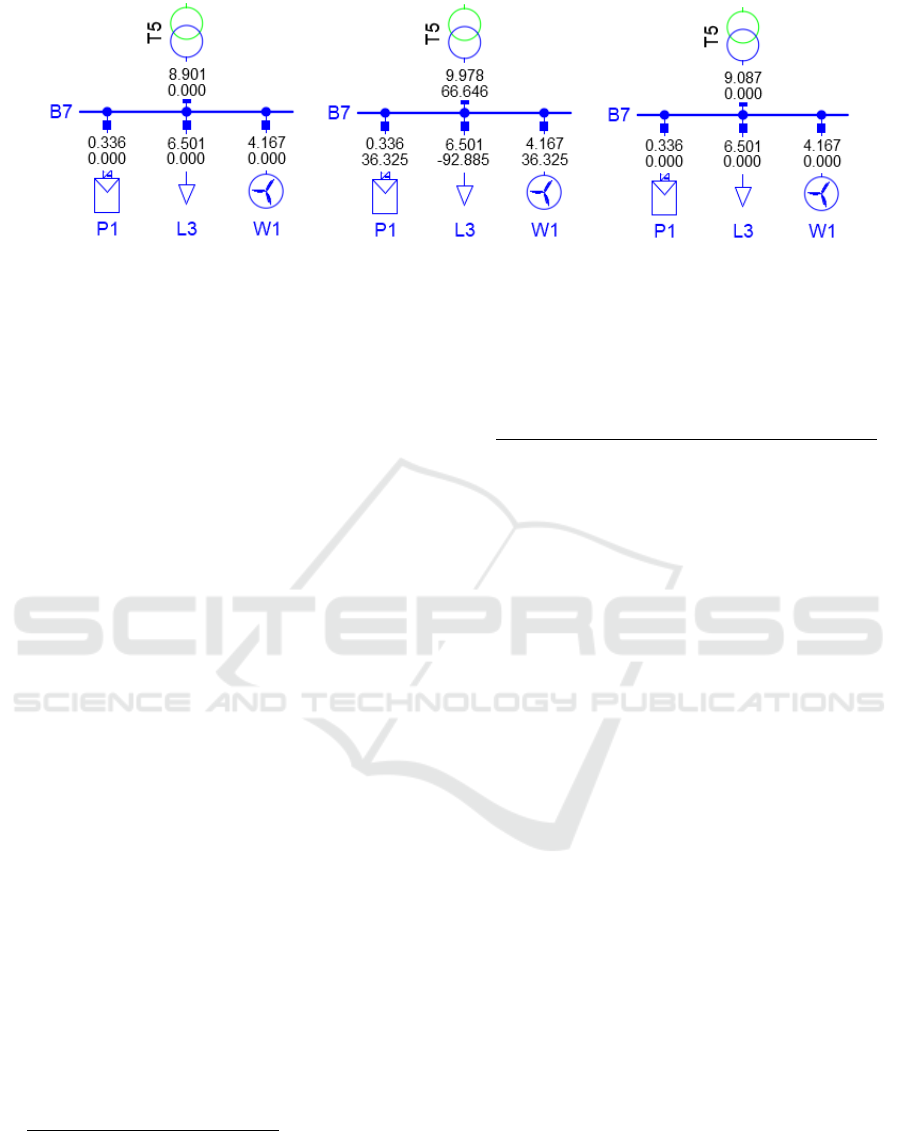
Figure 5: 5

harmonic order current flows obtained by using: the standard IEC model (left), the UPC model (middle), and the

UPC model assessed by standard IEC summation rule (right).

The differences between IEC and UPC model can be

explained by observing the use of summation rule,

that takes the cancellation effect between harmonic

sources into account.

In Table 6, the results obtained by applying IEC

model under different cases using a self-defined

summation exponent (i.e. value 1 was used for all

frequencies) are presented. The use of the self-

defined summation exponent leads to larger THDs

because it assumes that all harmonics are in-phase

(i.e. no cancellation effects), while the standard

coefficient implies cancellation effect with increasing

harmonic orders. On the other hand, in DPF, the UPC

model can also be processed using the IEC

summation rule, as long as one harmonic source is

using IEC model. Table 6 indicates that the THDs of

UPC model assessed by the standard IEC summation

rule (i.e. by setting L3 to use IEC model and other two

devices use UPC model) is close to the THDs

obtained from using the standard IEC model (results

of standard IEC model shown in Table 5). The UPC

model applying the standard IEC summation rule

considers both summation rule and harmonic phase

angles, therefore not matching the results obtained

with the standard IEC model.

To understand the causes of the discrepancies, it

is worthwhile to analyse the harmonic current flows

in detail. It is found that the summation of harmonic

currents produced by various sources at the low-

voltage side leads to different results when different

summation rules and harmonic source models are

applied. This is illustrated for the 5

harmonic current

as shown in Figure 5, where sources P1, L3 and W1

are considered. The total harmonic current magnitude

obtained for the standard IEC model is 8.901 A (i.e.

√

0.336

.

+ 6.501

.

+ 4.167

.

.

); for the UPC

model it is 9.978 A, obtained as |0.336 ∠36.325° −

6.501∠ − 92.885°+4.167∠36.325°|. Note that the

harmonic current injection of the load element of

UPC source model is considered in an opposite

direction of the IEC source model in DPF. The last

case in Figure 5 shows the UPC model assessed by

the standard IEC rule, considering both the standard

IEC summation exponent and the UPC angles, thus

leading to a total harmonic current of 9.087 A (i.e.



|0.336

∠

36.325

+4.167

∠

36.325

.

+6.501

.

.

When the self-defined summation exponent was used,

the above current flow equations were changed

accordingly.

Given the above results, the UPC model

considering harmonic phase angles may be preferable

under some circumstances, because it allows

modelling the harmonic phase angles in a flexible

way. On the contrary, the IEC model using the

standard summation exponent may put emphasis on

harmonic cancellation, while the phase angles are

fixed. Therefore, the UPC model will generally not

match exactly the standard IEC model, even if the

standard IEC summation rule is applied to the UPC

model. By adjusting the settings, the UPC model will

lead to results that are comparable to the IEC model,

as discussed in the next section.

3.2.3 Matching IEC and Equivalent UPC

Harmonic Current Model

After identifying the sources of discrepancies, the

following settings are proposed to improve the match

between the IEC model and the UPC model:

• The in-phase UPC model needs to be set as

follows: the three-phase angles (i.e. 𝜑





, 𝜑





and 𝜑





) of positive-sequence and triplen

orders in UPC model are set to 0°, −120° and

120°, while 0°, 120° and −120° are used for

negative-sequence orders. The use of such in-

phase UPC harmonic source model will not

consider harmonic cancellation effect and will

ensure that the same amount of harmonic

current injections is obtained when multiple

•

Modelling Renewable Energy Sources for Harmonic Assessments in DIgSILENT PowerFactory: Comparison of Different Approaches

137

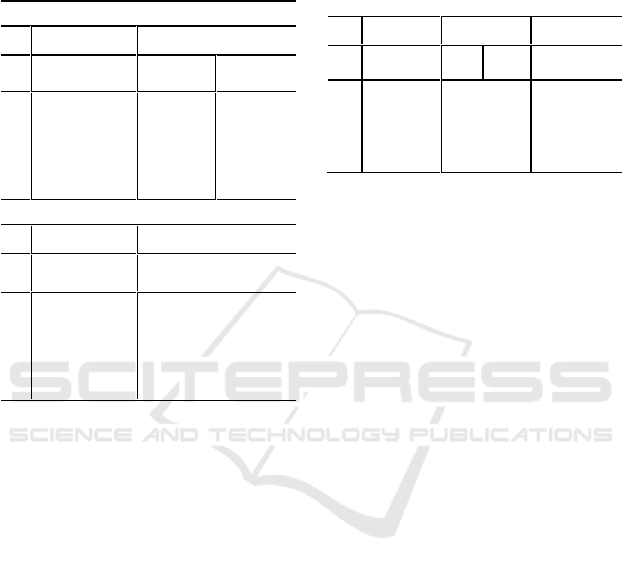
Table 7: THD results for self-defined IEC and in-phase

UPC modes under different study cases when using Yg-yg

transformers.

Three harmonic sources

Self-defined IEC

Model

In-Phase UPC Model

Bus

Case

4,5,6

(%)

Case

*,5*,6*

(%)

Case

4,5,6*

(%)

Case 6

3-Ph

(%)

B1 0.160 0.158

0.158 0.160

B2 0.620 0.613 0.613 0.620

B3 0.611 0.600 0.600 0.611

B4 0.698 0.690 0.690 0.698

B5 0.753 0.740 0.740 0.753

B6 0.745 0.732 0.732 0.745

B7 3.437 3.261 3.261 3.437

B8 0.753 0.740 0.740 0.753

B9 0.745 0.732 0.732 0.745

Seven harmonic sources

Self-defined IEC

Model

In-Phase UPC Model

Bus

Case

4,5,6

(%)

Case

4&6*

(%)

Case

(%)

Case 6

3-Ph

(%)

B1 0.257 0.243 0.243 0.248

1.001

0.918 0.918 0.931

1.008

0.934 0.935 0.960

1.110

0.987 0.986 1.005

1.166

0.998 1.000 1.030

1.176

1.015 1.016 1.044

3.647

3.196 3.201 3.391

1.328

1.028 1.028 1.114

1.371

1.046 1.046 1.172

Note the cases with ‘*’ label refer to the triplen harmonics are not

considered.

harmonic sources are connected to same

busbar (i.e. similarly to the IEC model

assessed by self-define IEC summation rule).

• The magnitude of the harmonic currents in the

UPC model is required to be set to a negative

value when modelling a load element.

• The Yg-yg transformer connection is needed

to avoid discrepancies at low-voltage busbars.

For example, different three-phase THD

values of UPC model for Case 6, and different

THDs of IEC and UPC models obtained from

different harmonic load flow solvers, as

discussed in 3.2.1

By using the settings above for the three harmonic

sources test, using the self-defined IEC and in-phase

UPC models lead to the same harmonic current

injection propagating to the upstream network. As

shown in Table 7 (bold values), the THDs obtained

from using in-phase UPC model are same to the self-

defined IEC model, except the UPC model under

Case 4 and 5 (because these cases are ignoring the

triplen harmonics). When triplen harmonics were

Table 8: THDs of self-defined IEC and in-phase UPC

models for different cases when length of transmission lines

and phase-shift of transformers are set to zero and using Yg-

yg transformers (seven harmonic sources).

Self-defined

IEC Model

In-Phase UPC

Model*

In-Phase UPC

Model

Bus

Case

4,5,6

(

)

Case

4,5,6

(%)

Case 6

3-Ph

(%)

Case

4,5,6

(%)

Case 6

3-Ph (%)

B1 0.387 0.368 0.387 0.366 0.387

B2 1.518 1.444 1.518 1.439 1.518

B3 1.518 1.444 1.518 1.439 1.518

B4 1.518 1.444 1.518 1.439 1.518

B5 1.518 1.444 1.518 1.439 1.518

B6 1.518 1.444 1.518 1.439 1.518

B7 4.974 4.748 4.974 4.708 4.974

B8 1.854 1.723 1.854 1.719 1.854

B9 1.992 1.813 1.992 1.808 1.992

‘In-phase UPC model*’ means the UPC model is assessed by self-

defined summation rule, and the ‘6*’ is the case 6 without

considering triplen harmonics.

ignored in the IEC models, the THDs were same to

the UPC model under different cases (see Table 7).

When seven harmonic sources – 3 loads, 2 PVs

and 2 WTGs – located at different busbars were

considered, the THD values of self-defined IEC and

in-phase UPC model were not matching although the

differences were small (see Table 7). Note that the

THDs of in-phase UPC model under Case 5 were not

exactly the same as in Case 4 and Case 6*, because

the solver in Case 5 considers positive-sequence

impedance for all harmonic orders.

Nevertheless, it is possible to match the results

obtained from the IEC model with the self-defined

summation exponent (i.e. 1 for all frequencies) by

using the proposed in-phase model if the length of the

transmission lines and the phase-shift of the

transformers are considered to be zero. In this way,

the diversity due to the network impedance is not

considered, therefore the comparison between

different harmonic modelling approaches and

harmonic load flow solvers is straightforward. The

voltage THD results in Table 8 show that the use of

in-phase UPC model produce the same THDs (the

bold values) as the use of self-defined IEC model for

Case 6 under the specified system conditions.

Moreover, Table 8 shows that the UPC model

assessed by IEC summation rule with self-defined

summation exponent (i.e. ‘In-Phase UPC*’) is able to

produce the same result for Case 6 (see bold values in

Table 8). The differences between In-Phase UPC and

In-Phase UPC under Case 4, 5 and 6* are because the

device L3 in the case In-Phase UPC* was using IEC

model that takes triplen harmonics into account.

Based on the results above, even with the

proposed settings, the in-phase UPC model does not

allow exact match of the IEC model results obtained

by applying the standard summation rule when

SIMULTECH 2021 - 11th International Conference on Simulation and Modeling Methodologies, Technologies and Applications

138

multiple harmonic sources are located at different

busbars. This is because the UPC model takes into

account the cancellation caused by the network

impedance (i.e. superposition law): more specifically,

it was found that the harmonics propagating to the

network through the transmission lines and phase-

shifting transformers result in harmonic phase shift

when using the UPC model. On the contrary, the

standard IEC model summation rule accounts for the

effect of harmonic cancellation from the harmonic

source injections and the effect of network impedance,

irrespective of the transformer phase shift.

4 CONCLUSIONS

This paper addressed different approaches in

modelling unbalanced systems with large penetration

of RESs for the purpose of harmonic studies. Two

aspects were considered: frequency scans and

harmonic penetration studies.

The frequency scans indicated that the single-

phase and three-phase network impedance

characteristics were not affected by the harmonic

models and the number of harmonic sources, as well

as the use of balanced and unbalanced solver.

Various harmonic settings in DPF were tested to

solve harmonic power flow using the IEC and UPC

model. the discrepancies caused by the two models

and harmonic load flow solvers have been analysed

and clarified by comparing different cases. In

addition, the possibility and requirement of modelling

equivalent IEC model by using the UPC model have

been proposed and verified.

Finally, it was concluded that the UPC model and

the unbalanced harmonic load flow should be

considered for harmonic analysis for certain

operating conditions, for example (1) in stochastic

harmonic analysis, (2) where it is deemed that the

generic IEC summation rule may lead to

underestimation or overestimation of harmonic

levels, as it assumes a ‘standard’ cancellation of

harmonic that may not take place in the practice.

When power converter-based devices, such as RESs,

are considered, it is recommended to adopt the UPC

model that accurately considers harmonic magnitude

and phase. In this way, the harmonic cancellation

effect is considered properly, and thus the harmonic

assessment is more accurate and reliable.

Future work will include: developing a frequency-

dependent Norton admittance model to be used with

the UPC harmonic current source; applying this

model to a larger network representing a portion of

the UK transmission grid and studying increasing

levels of RESs and their impact on harmonic levels

on the system.

ACKNOWLEDGEMENTS

The authors acknowledge the support of the UK

Engineering and Physical Sciences Research Council

(EPSRC); Project EP/T013206/1.

REFERENCES

Ambrož, B., Boštjan, B., Aljaž, Š., Mari, L., Jako, K., &

Kai, S. (2017). Simulation Models for Power-Quality

Studies in Power-Electronics Rich Power Networks-

Deliverable 5.2. MIGRATE – Massive InteGRATion of

Power Electronic Devices, 1–323.

Bećirović, E., Jovica, V. M., Simon, H., Maren, K., Kai, S.,

& Dejan, M. (2018). Propagation of PQ disturbances

Through The Power Networks - Deliverable 5.3.

MIGRATE – Massive InteGRATion of Power

Electronic Devices, 1–154.

Cherian, E., Bindu, G. R., & Chandramohanan, P. S.

(2016). Pollution Impact of Residential Loads on

Distribution System and Prospects of DC Distribution.

Engineering Science and Technology, an International

Journal, 19(4), 1655–1660.

DIgSILENT. (2020a). PowerFactory 2020.

https://www.digsilent.de/en/powerfactory.html

DIgSILENT. (2020b). PowerFactory 2020 User Manual.

889–906. https://www.digsilent.de/en/powerfactory.

html

Elkholy, A. (2019). Harmonics Assessment and

Mathematical Modeling of Power Quality Parameters

for Low Voltage Grid Connected Photovoltaic Systems.

Solar Energy, 183, 315–326.

Eltouki, M., Rasmussen, T. W., Guest, E., Shuai, L., &

Kocewiak, Ł. (2018). Analysis of Harmonic

Summation in Wind Power Plants Based on Harmonic

Phase Modelling and Measurements. 17th International

Wind Integration Workshop, 1–7.

Energy Networks Association. (2020). Harmonic Voltage

Distortion and the Connection of Non-Linear and

Resonant Plant and Equipment to Transmission

Systems and Distribution Networks in the United

Kingdom. ENA Engineering Recommendation G5, 5.

Energyiforsk. (2018). Harmonics and Wind Power. Daphne

Schwanz, Math Bollen, Lulea University of Technology,

1–42.

Erik, J., & Leigh, S. H. (2016). Power Quality Assessment

of Solar Photovoltaic Inverters. Sustainable

Technologies Evaluation Program, Toronto and

Region Conservation Authority, Toronto, Ontario, 1–

58.

Ghassemi, F., & Koo, K. (2010). Equivalent Network for

Wind Farm Harmonic Assessments. IEEE Transactions

on Power Delivery, 25(3), 1808–1815.

Modelling Renewable Energy Sources for Harmonic Assessments in DIgSILENT PowerFactory: Comparison of Different Approaches

139

Herraiz, S., Sainz, L., & Clua, J. (2003). Review of

Harmonic Load Flow Formulations. IEEE Transactions

on Power Delivery, 18(3), 1079–1087.

IEC TR 61000-3-6. (2008). Electromagnetic Compatibility,

Limits – Assessment of Emission Limits for The

Connection of Distorting Installations to MV, HV and

EHV Power Systems.

IEEE Power and Energy Society. (2014). IEEE

Recommended Practice and Requirements for

Harmonic Control in Electric Power Systems. IEEE

Std. 519-2014.

Jensen, C. F. (2018). Harmonic Background Amplification

in Long Asymmetrical High Voltage Cable Systems.

Electric Power Systems Research, 160, 292–299.

Koo, K. L., & Emin, Z. (2016). Comparative Evaluation of

Power Quality Modelling Approaches for Offshore

Wind Farms. 5th IET International Conference on

Renewable Power Generation (RPG), 1–7.

Medina, A., Segundo, J., Ribeiro, P., Xu, W., Lian, K. L.,

Chang, G. W., Dinavahi, V., & Watson, N. R. (2013).

Harmonic Analysis in Frequency and Time Domain.

IEEE Transactions on Power Delivery, 28(3), 1813–

1821.

Mendonça, G. A., Pereira, H. A., & Silva, S. R. (2012).

Wind Farm and System Modelling Evaluation in

Harmonic Propagation Studies. Renewable Energy and

Power Quality Journal, 1(10), 647–652.

National Grid ESO. (2019). Future Energy Scenarios 2019.

http://fes.nationalgrid.com/fes-document/

Oliver, A., Liam, M., Griffiths, F., Shafiu, A., & Forooz, G.

(2018). Subgroup Report – Harmonics Above 50th.

ENA Engineering Recommendation G5.

Preciado, V., Madrigal, M., Muljadi, E., & Gevorgian, V.

(2015). Harmonics in A Wind Power Plant. IEEE

Power and Energy Society General Meeting, 1–5.

Preda, T. N., Uhlen, K., & Nordgard, D. E. (2012).

Instantaneous Harmonics Compensation Using Shunt

Active Filters in A Norwegian Distribution Power

System With Large Amount of Distributed Generation.

3rd IEEE International Symposium on Power

Electronics for Distributed Generation Systems

(PEDG), 153–160.

Rampinelli, G. A., Gasparin, F. P., Bühler, A. J.,

Krenzinger, A., & Chenlo Romero, F. (2015).

Assessment and Mathematical Modeling of Energy

Quality Parameters of Grid Connected Photovoltaic

Inverters. Renewable and Sustainable Energy Reviews,

52, 133–141.

Rauma, K. (2012). Electrical Resonances and Harmonics in

a Wind Power Plant. In Aalto University School of

Electrical Engineering Kalle.

Robinson, D. (2003). Harmonic Management in MV

Distribution Systems. University of Wollongong.

Working Group JWC-C4/B4.38. (2019). Network

Modelling for Harmonic Studies. CIGRE, 1–241.

Working Group JWG-C4/C6.29. (2016). Power Quality

Aspects of Solar Power. CIGRE, 1–109.

SIMULTECH 2021 - 11th International Conference on Simulation and Modeling Methodologies, Technologies and Applications

140