Vaccination and Time Limited Immunization for SARS-CoV-2 Infection
Paolo Di Giamberardino
a
and Daniela Iacoviello
b
Dept. Computer, Control and Management Engineering Antonio Ruberti, Sapienza University of Rome,
via Ariosto 25, 00185 Rome, Italy
Keywords:
COVID–19, Epidemic Model, Vaccination, Reinfection.
Abstract:
The paper aims at a discussion of the effects of the containment measures against COVID-19 through the anal-
ysis of the reproduction number. Starting from a mathematical model in which several controls are considered,
including the vaccination, and introducing also an hypotised limited duration of the immunity acquired both
from vaccine and from healing from the illness, the steady state behaviour, both in the uncontrolled and in
the controled cases is studied. The expressions for the basic reproduction number and the actual reproduction
number under control actions are computed by means of the next generation matrix approach. This function is
numerically investigated, showing some graphs which illustrate, qualitatively and quantitatively, in an intuitive
way the positive effects of the controls and the negative contribution of the absence of a lifetime immunization
from virus.
1 INTRODUCTION
Mathematical modelling of epidemics spread is a ba-
sic tool for prediction of different scenarios and for
the definition of suitable control actions aiming at the
virus containment.
Compartmental systems are usually adopted;
since the pioneering work (Kermack and McK-
endrick, 1927), all of them consider at least the com-
partment of susceptible individuals S that can get in-
fection, the infected ones I which can transmit the
virus, and the recovered patients R healed from the
illness (SIR model).
Richer descriptions include additional classes like,
for example, the exposed patients E, if the virus has
a significant incubation time, or people that lose im-
munity after infection C. Moreover, for the descrip-
tion of each specific infection, particular classes are
included. Descriptions and discussions on epidemic
modelling can be found in (Daley and Gani, 1999;
Martcheva, 2015).
For the COVID-19, the more or less dangerous-
ness of the evolution of the illness for different pa-
tients, going from asymptomatic ones to people re-
quiring long stay in intensive care, and the variability
of the death rate according to the age or the presence
of comorbidities, motivated the introduction of addi-
a
https://orcid.org/0000-0002-9113-8608
b
https://orcid.org/0000-0003-3506-1455
tional compartments to take into account all these pos-
sible levels of infection and therapeutic needs. De-
spite the quite limited time since the beginning of
this disease, the list of models introduced could be
long. Among the first models designed specifically
for the COVID-19 case there is (Tang et al., 2020),
where the pre-symptomatic infectious (A), the hospi-
talized (H), the quarantined susceptible (Sq), the iso-
lated exposed (Eq) and the isolated infected (Iq) com-
partments are considered. In (Di Giamberardino and
Iacoviello, 2021) the quarantined compartment con-
taining temporarily isolated individuals is added and
the infected people are divided into symptomatic and
asymptomatic ones, analysing the role of the latter. In
(Gumel et al., 2021) the infected patients are divided
into asymptomatic (Ia), symptomatic (Is), and hospi-
talized (Ih) classes. Sometimes the population is also
divided into categories, often age based (Di Giamber-
ardino et al., 2020), to analyse the effects of the epi-
demics on the different groups.
Models allow to study the actual spread dynamics,
to predict its behaviour for different scenarios and to
help in the designing of control laws or, at least, in
supporting political and social decisions for epidemic
containment. A compact description of the epidemic
dangerousness, usually adopted for driving govern-
ments interventions, is the so called basic reproduc-
tion number R , representing an important indicator
commonly used for characterising the velocity of dif-
fusion of one epidemic, so measuring its impact on
Di Giamberardino, P. and Iacoviello, D.
Vaccination and Time Limited Immunization for SARS-CoV-2 Infection.
DOI: 10.5220/0010578106090619
In Proceedings of the 18th International Conference on Informatics in Control, Automation and Robotics (ICINCO 2021), pages 609-619
ISBN: 978-989-758-522-7
Copyright
c
 2021 by SCITEPRESS – Science and Technology Publications, Lda. All rights reserved
609

the population in terms of rate of increment of in-
fected individuals. It is defined as the number of in-
dividuals directly infected by one infective person as-
sumed as the only infective subject in all the popu-
lation (Diekmann et al., 1990; Dietz, 1993; Perasso,
2018; Zhao et al., 2020; Katul et al., 2020).
This definition is purely theoretical, since the esti-
mation of such a quantity is performed when the dis-
ease is already present, the number of infective per-
sons is much larger than one and some intervention
policies are already adopted. So, there are statisti-
cal approaches to estimate R
0
from data series of
infected individuals (Dietz, 1993). The computation
does not follow a unique approach, so there are sev-
eral procedures for its computations which differ for
statistical assumptions. In (Billah et al., 2020) such
differences are presented and discussed. An estima-
tion can also be computed on the basis of the model of
the epidemics dynamics making use of the next gener-
ation matrix (Diekmann et al., 2010; van den Driess-
che, 2017; Perasso, 2018). The use of a model to
compute the basic reproduction number can be help-
ful for the evaluation of the influence of the param-
eters to its value. Moreover, if the controls are con-
sidered too, a controlled reproduction number can be
introduced to evaluate also their effects on the virus
spread; this means that it is possible to establish a re-
lationship, also in a quantitative way, between con-
trols and reproduction number value, so supporting
the evaluation of the effects of interventions (van den
Driessche, 2017).
In the present work, the model proposed in (Di Gi-
amberardino and Iacoviello, 2021) is considered as a
validated starting point from which additional effects
can be studied. In particular, in the present paper, the
vaccination u
6
is introduced, being at present a rel-
evant control action not sensibly present yet at time
of (Di Giamberardino and Iacoviello, 2021). More-
over, based on the observation that the immunization
produced by a vaccine seems to have a time limited
duration, the lost of antibodies and then the possible
reinfection is also considered (ρR), making the rate
of vaccination an important issue to be faced. The
analysis of the combined and contrasting effects of the
modelled intervention actions and the end of the im-
munization is performed by means of the dependency
of the basic reproduction number from such quanti-
ties. In Section 2 the model is introduced and briefly
described while its equilibrium and stability charac-
teristics are addressed in Section 3. In view of the
analysis for the controlled case, the effects of the in-
puts on the equilibrium points and their stability are
shown in Section 4. The influences of the controls on
the reproduction number are studied and discussed in
Section 5. Some concluding comments in Section 6
end the paper.
2 THE MATHEMATICAL MODEL
The mathematical model here adopted is the one in-
troduced in (Di Giamberardino and Iacoviello, 2021),
modified adding the vaccination control, denoted by
u
6
, and the limited time of immunity for healed and
vaccinated individuals, introduced by means of a time
constant ρ. Moreover, since the work is mainly fo-
cused on the analysis of the opposite effects of the
vaccination and the lost of immunization with conse-
quent possibility of reinfection, the model is simpli-
fied neglecting the quarantined class, also in view of
the relatively low number of individuals in such a con-
dition and, then, their negligible effect with respect of
the vaccination process.
The scheme in Figure 1 describes the compart-
ment model introduced. Solid lines/arrows denote the
natural flux of the infection evolution, from the class
S of susceptible to the class R of the recovered in-
dividuals, and from the recovered to the susceptible
classes for the lost of immunity; this natural flux in-
cludes also the dotted arrows, representing the death
people from all the classes. Dashed lines represent the
control actions, whose description is provided below.
Figure 1: Block scheme of the compartmental model stud-
ied.
The resulting dynamics is described by the equa-
tions
˙
S = B − β(1 − u
2
)SI
C
− vu
6
S + ρR − d
S
S
˙
E = β(1 − u
2
)SI
C
− au
1
E − kE − d
E
E
˙
I
C
= kE − au
1
I
C
− h
1
I
C
− h
2
I
C
− d
I
C
I
C
˙
I
Q
= au
1
(E + I
C
) + h
1
I
C
− (γ + ηu
3
)I
Q
− d
I
Q
(1 − u
4
)I
Q
˙
R = h
2
I
C
+ (γ + ηu
3
)I
Q
+ vu
6
S − ρR − d
R
R
(1)
ICINCO 2021 - 18th International Conference on Informatics in Control, Automation and Robotics
610

where all the state variables represent the number of
individuals in the corresponding class. They are
S the susceptible individuals;
E the exposed ones, already infected but not yet in-
fective since the virus is in its incubation period;
the time constant for incubation condition is 1/k
I
C
the infected patients without symptoms; they are
infective and then are the responsible of the dis-
ease spread. They can remain asymptomatic for
all the illness course till healing, with time rate
h
2
, or can start to have some symptoms, with rate
h
1
;
I
Q
the diagnosed infected patients which are isolated
and then cannot transmit the virus even if infec-
tive. Patients in this class are the ones that can re-
ceive medical treatment both against the infection,
u
3
, like antivirals, monoclonal antibodies and so
on, so increasing the recovering rate, and for re-
ducing the secondary diseases or complications
even to intensive care support, u
4
, reducing the
mortality;
R the immune individuals which are supposed to be
neither infected nor infectious, composed by the
recovered patients, the ones healed spontaneously
or after therapy, and the vaccinated individuals.
They are protected from infection for a limited
time period after which they return to be suscepti-
ble with a time rate ρ.
In the model are also present a constant rate of new-
borns B, the transmission rate β from which the epi-
demic spread depends, the spontaneous rate of heal-
ing of diagnosed patients γ, and the death rates d
∗
,
possibly different for each class. Along with these pa-
rameters, in the model there are present the control u
2
,
which acts on the individual interactions by means of
social restrictions, use of masks, till lock down peri-
ods, the input au
1
representing the effects of the tests
for infection detection, and the vaccination rate vu
6
.
Note that vaccination affects susceptible individuals
only since E and I
C
, even if vaccinated, do not leave
their classes because they do not change their infec-
tive status.
A short analysis of dynamical characteristics is
provided in next Subsection 3 to show the differences
with respect to the original model.
3 EQUILIBRIUM CONDITIONS
In the system analysis, the computation of the equi-
librium points and the study of their stability is a
preliminary step for understanding the qualitative be-
haviour of the dynamics. According to the classi-
cal approach, the uncontrolled system is considered
(u
i
= 0, i = 1, 2,. .. ,6).
3.1 Equilibrium Points
The equilibrium points are obtained setting equal to
zero the variations in (1). Then, the solutions of
B − βS
e
I
e
C
− d
S
S
e
+ ρR
e
= 0 (2)
βS
e
I
e
C
− (k + d
E
)E
e
= 0 (3)
kE
e
− (h
1
+ h
2
+ d
I
C
)I
e
C
= 0 (4)
h
1
I
e
C
− γI
e
Q
− d
I
Q
I
e
Q
= 0 (5)
h
2
I
e
C
+ γI
e
Q
− d
R
R
e
− ρR
e
= 0 (6)
must be computed. The system is a slight variation
of the one considered in (Di Giamberardino and Ia-
coviello, 2021), but the presence of the reinfection
term ρR plays a relevant role for changing the results.
To find the solutions, from (4) the expression
E
e
=
m
1
k
I
e
C
(7)
can be obtained, with m
1
= h
1
+ h
2
+ d
I
C
; moreover,
setting m
2
= k + d
E
and substituting (7) into (3), one
gets

βS
e
−
m
1
m
2
k

I
e
C
= 0 (8)
The solution I
e
C
= 0 of (8), once substituted into (7)
and evaluated (5), characterises the solution without
infected individuals, and then the absence of infec-
tion. It corresponds to the so called epidemic free
condition, corresponding to the equilibrium with all
the infected classes empty. Computing the two re-
maining components the first equilibrium point P
e
1
is
obtained, whose expression is
P
e
1
=

S
e
1
E
e
1
I
e
C1
I
e
Q1
R
e
1

T
=

B
d
S
0 0 0 0

T
(9)
The second solution of (8) is
S
e
=
m
1
m
2
βk
(10)
Then, from (5) the relationship
I
e
Q
=
h
1
(γ + d
I
Q
)
I
e
C
(11)
is obtained and, used in (6), one has
R
e
=
h
2
(γ + d
I
Q
) + γh
1
(d
R
+ ρ)(γ + d
I
Q
)
I
e
C
(12)
Vaccination and Time Limited Immunization for SARS-CoV-2 Infection
611

Making use of all such relationships in (2), the equa-
tion
B − d
S
S
e
− βS
e
− ρ
h
2
(γ + d
I
Q
) + γh
1
(d
R
+ ρ)(γ + d
I
Q
)
!
I
e
C2
= 0
(13)
is obtained, which, once solved, gives the values for
the component I
e
C
6= 0 of the second equilibrium point.
The non null number of infected individuals at the
equilibrium, which means that in these conditions the
epidemic is always present in the population, moti-
vates the definition of endemic usually given to such
a condition. Denoting by
P
e
2
=

S
e
2
E
e
2
I
e
C2
I
e
Q2
R
e
2

T
(14)
the equilibrium point, S
e
2
corresponds to (10) and,
from (13)
I
e
C2
=
B − d
S
S
e
2

βS
e
2
− ρ
h
2
(γ+d
I
Q
)+γh
1
(d
R
+ρ)(γ+d
I
Q
)

(15)
In order to be an admissible value for the equilibrium
point, I
e
C2
must be non negative. The resulting condi-
tions are



B − d
S
m
1
m
2
βk
> 0
m
1
m
2
k
− ρ
h
2
(γ+d
I
Q
)+γh
1
(d
R
+ρ)(γ+d
I
Q
)
> 0
(16)
or



B − d
S
m
1
m
2
βk
< 0
m
1
m
2
k
− ρ
h
2
(γ+d
I
Q
)+γh
1
(d
R
+ρ)(γ+d
I
Q
)
< 0
(17)
The first can be written as



m
1
m
2
k
<
βB
d
S
m
1
m
2
k
> ρ
h
2
(γ+d
I
Q
)+γh
1
(d
R
+ρ)(γ+d
I
Q
)
(18)
and it is satisfied if and only if
ρ
h
2
(γ + d
I
Q
) + γh
1
(d
R
+ ρ)(γ + d
I
Q
)
<
m
1
m
2
k
<
βB
d
S
(19)
while the second holds if and only if



m
1
m
2
k
>
βB
d
S
m
1
m
2
k
< ρ
h
2
(γ+d
I
Q
)+γh
1
(d
R
+ρ)(γ+d
I
Q
)
(20)
that is
βB
d
S
<
m
1
m
2
k
< ρ
h
2
(γ + d
I
Q
) + γh
1
(d
R
+ ρ)(γ + d
I
Q
)
(21)
It must be noted that in this case, the presence of the
reinfection factor ρ affects the existence of the en-
demic equilibrium point, introducing one distinction
from the case discussed in (Di Giamberardino and Ia-
coviello, 2021). Clearly, if ρ = 0, the conditions re-
duce to one only, the same as in (Di Giamberardino
and Iacoviello, 2021)
B − d
S
S
e
= B − d
S
m
1
m
2
βk
> 0 (22)
3.2 Stability Analysis
The local stability of the two equilibrium points pre-
viously found is now studied. The Jacobian for the
given dynamics in the uncontrolled case, evaluated in
the equilibrium point P
e
1
is
J(P
e
1
) =


−d
S
J
1,2
0
A
1,1
0
A
2,1
A
2,2


(23)
with
A
1,1
=

−m
2
βS
e
1
k −m
1

(24)
A
2,2
=

−(γ+d
I
Q
) 0
γ −(ρ+d
R
)

(25)
The eigenvalues
λ
1
= −d
S
, λ
2
= −γ + d
I
Q
(26)
λ
3
= −(ρ + d
R
) (27)
are directly obtained thanks to the structure of the ma-
trix (23), and are all real negative. The remaining two,
the ones of matrix A
1,1
, are the solutions of the char-
acteristic equation
λ
2
+ (m
1
+ m
2
)λ + (m
1
m
2
− kβS
e
1
) = 0 (28)
For the Descartes’ rule of signs, they have a negative
real part if and only if
m
1
m
2
− k βS
e
1
> 0 (29)
Then, the fulfilment of condition (29) implies the lo-
cal asymptotic stability of the equilibrium point P
e
1
.
As far as P
e
2
is concerned, the Jacobian evaluated
in such a point assumes the expression
J(P
e
2
) =



−βI
e
C2
−d
S
0 −βS
e
2
0 ρ
βI
e
C2
−m
2
βS
e
2
0 0
0 k −m
1
0 0
0 0 h
1
−(γ+d
I
Q
) 0
0 0 h
2
γ −(ρ+d
R
)



(30)
Its characteristic equation is given by
p(λ) = λ
5
+C
4
λ
4
+C
3
λ
3
+C
2
λ
2
+C
1
λ +C
0
= 0
(31)
with
C
4
= βI
e
C2
+ d
S
+ m
1
+ m
2
+ ρ + d
R
+ γ + d
I
Q
C
3
= (βI
e
C2
+ d
S
)(m
1
+ m
2
+ γ + d
I
Q
+ ρ + d
R
)
+(γ + d
I
Q
+ ρ + d
R
)(m
1
+ m
2
) + (γ +d
I
Q
)(ρ + d
R
)
C
2
= (ρ + d
R
+ γ + d
I
Q
)(βI
e
C
+ d
S
)(m
1
+ m
2
)+
+(βI
e
C
+ d
S
+ m
1
+ m
2
)(ρ + d
R
)(γ + d
I
Q
)+
+βI
e
C2
m
1
m
2
ICINCO 2021 - 18th International Conference on Informatics in Control, Automation and Robotics
612

C
1
= βI
e
C2
m
1
m
2
(γ + d
I
Q
+ ρ + d
R
) − kh
2
ρβI
e
C2
+(m
1
+ m
2
)(βI
e
C2
+ d
S
)(γ + d
I
Q
)(ρ + d
R
)
C
0
= βI
e
C2
m
1
m
2
(γ + d
I
Q
)(ρ + d
R
)
−ρkβI
e
C2

h
1
γ + h
2
(γ + d
I
Q
)

A necessary condition for having all the roots with
negative real part is that all the coefficients C
i
are pos-
itive. From the non negativeness of the parameters, it
is possible to see that C
4
> 0, C
3
> 0 and C
2
> 0. Also
C
1
> 0 because, recalling the expressions for m
1
and
m
2
, after some manipulations it is possible to get the
expression
C
1
= βI
e
C2
m
1
m
2
(γ + d
I
Q
+ d
R
)
+ρβI
e
C2
((h
1
+ h
2
+ d
I
C
)d
E
+ (h
1
+ d
I
C
)k)
+(m
1
+ m
2
)(βI
e
C2
+ d
S
)(γ + d
I
Q
)(ρ + d
R
)
As far as C
0
is concerned, its positiveness is guaran-
teed if and only if
m
1
m
2
k
− ρ
h
2
(γ + d
I
Q
) + γh
1
(d
R
+ ρ)(γ + d
I
Q
)
> 0 (32)
since simple computations allows to write
C
0
= βkI
e
C2
(γ + d
I
Q
)(ρ + d
R
)× (33)
m
1
m
2
k
− ρ

h
1
γ + h
2
(γ + d
I
Q
)

(γ + d
I
Q
)(ρ + d
R
)
!
(34)
The necessary and sufficient conditions for the
polynomial to have roots with negative real part can
be obtained making use of the Rooth–Hurwitz crite-
rion. It requires the fulfilment of the following condi-
tions
C
4
> 0 (35)
C
6
= C
3
C
4
−C
2
> 0 (36)
C
8
= C
2
C
6
−C
4
C
7
> 0 (37)
C
9
= C
7
(C
2
C
6
−C
4
C
7
) −C
0
C
6
> 0 (38)
where
C
7
= C
1
C
4
−C
0
; (39)
Once again, the presence of the reinfection term
makes the computations much more long and difficult
with respect to the case in (Di Giamberardino and Ia-
coviello, 2021). Since they are not so meaningful as
for the epidemic free equilibrium, the computations
are not here explicitly performed.
The consistence of the present conditions can be
verified noticing that, setting ρ = 0, the polynomial
(31) can be written as
p(λ) = (ρ +d
R
)(γ + d
I
Q
)p
2
(λ) (40)
where
p
2
(λ) = λ
3
+
˜
C
2
λ
3
+
˜
C
1
λ +
˜
C
0
(41)
with
˜
C
2
= βI
e
C2
+ d
S
+ m
1
+ m
2
(42)
˜
C
1
= (m
1
+ m
2
)βI
e
C2
(43)
˜
C
0
= m
1
m
2
βI
e
C2
(44)
and it is possible to verify that the Rooth–Hurwitz
conditions C
0
> 0, C
2
> 0 and C
1
C
2
− C
0
are satis-
fied provided that I
e
C2
0 is admissible, i.e. condition
(16) or (17) hold.
3.3 The Basic Reproduction Number
R
0
Starting from the model (1), the basic reproduction
number is here computed making use of the next gen-
eration matrix (Diekmann et al., 2010).
This approach, in the present case, brings to the
following steps. The part of the dynamics directly in-
volved in the contagious or in the secondary infec-
tions is the one which characterises the state variables
Z =

E I
C
I
Q

T
(45)
The corresponding part of the dynamics must be par-
titioned into the part F which describes the first in-
fection, that is the transmission from one infected to a
susceptible individual
F =

βSI
C
0 0

T
(46)
and the part −V which describes the disease propa-
gation
V =


m
2
E
−kE + m
1
I
C
−h
1
I
C
+ (γ + d
I
Q
)I
Q


(47)
The following matrices can be computed
F =
∂F
∂Z




P
e
1
=


0 βS 0
0 0 0
0 0 0


(48)
V =
∂V
∂Z




P
e
1
=


m
2
0 0
−k m
1
0
0 −h
1
(γ + d
I
Q
)


(49)
The estimation of R
0
is then given by the eigen-
vector with the greatest modulus of the matrix FV
−1
.
Then,
V
−1
=



1
m
2
0 0
k
m
1
m
2
1
m
1
0
∗ ∗
1
γ+d
I
Q



(50)
FV
−1
=


kβS
e1
m
1
m
2
βS
e1
m
1
0
0 0 0
0 0 0


(51)
and the basic reproduction number is given by
R
0
=
kβS
e1
m
1
m
2
=
kβB
m
1
m
2
d
S
(52)
Vaccination and Time Limited Immunization for SARS-CoV-2 Infection
613

4 ANALYSIS FOR THE CASE OF
CONSTANT CONTROLS
The classical stability analysis performed in the previ-
ous Section can be enriched including the possibility
of having non null controls, making the equilibrium
points and their stability conditions a function of the
inputs. This analysis can be very important since once
the relationships between the actions performed and
the epidemic evolution are quantitatively defined, it
is possible to analyse different scenarios according to
social and political choices of intervention. For sake
of length and complexity in the expressions involved,
the analysis is mainly focused on the epidemic free
equilibrium existence and stability, since it is the de-
sired condition to which the evolution is intended to
be driven, and also because of its relationship with the
important parameter R
0
.
To compute the equilibrium points, the system
B − β
u
SI
C
− c
1
S + ρR = 0 (53)
β
u
SI
C
− c
2
E = 0 (54)
kE − c
3
I
C
= 0 (55)
au
1
(E + I
C
) + h
1
I
C
− c
4
I
Q
= 0 (56)
h
2
I
C
+ (γ + ηu
3
)I
Q
+ vu
6
S − (ρ + d
R
)R = 0 (57)
with
β
u
= β(1 − u
2
) (58)
c
1
= vu
6
+ d
S
(59)
c
2
= au
1
+ m
2
(60)
c
3
= au
1
+ m
1
(61)
c
4
= ((γ + ηu
3
) + d
I
Q
(1 − u
4
)) (62)
must be solved. It is the same as (2)–(6) with all the
controls present. From (55), one has
E =
c
3
k
I
C
(63)
that, used in (54), gives

β
u
S −
c
2
c
3
k

I
C
= 0 (64)
From this equation the two roots
I
C
= 0 S =
c
2
c
3
kβ
u
(65)
are obtained. Making use of the first one, for (63) one
gets E = 0. With the null values for E and I
C
, the
remaining equations to be solved are
B − c
1
S + ρR = 0 (66)
−c
4
I
Q
= 0 (67)
(γ + ηu
3
)I
Q
+ vu
6
S − (ρ + d
R
)R = 0 (68)
from which the value I
Q
= 0 is obtained. As a conse-
quence, the relationship
R =
vu
6
(ρ + d
R
)
S (69)
holds and, by substitution, the equation
B −

c
1
S − ρ
vu
6
(ρ + d
R
)

S = 0 (70)
is obtained. Once solved, all the components of the
equilibrium point, here denoted by P
e1
u
, are computed.
One has
S
e1
u
=
B

c
1
− ρ
vu
6
(ρ+d
R
)

(71)
which can be rewritten as
S
e1
u
=
B
d
R
(ρ+d
R
)
vu
6
+ d
S
(72)
which, by (69), yields
R
e1
u
=
Bvu
6
d
R
vu
6
+ d
S
(ρ + d
R
)
(73)
so getting the first equilibrium point
P
e1
u
=

B
d
R
(ρ+d
R
)
vu
6
+d
S
0 0 0
Bvu
6
d
R
vu
6
+d
S
(ρ+d
R
)

(74)
Also for the controlled case, the point P
e1
u
, charac-
terised by the absence of infected individuals (I
e1
Cu
= 0,
E
e1
u
= 0 and I
e1
Qu
= 0), can be denoted as epidemic free
equilibrium.
For the second solution, with S
e2
u
as in (65), from
(56) one gets
I
Q
=

au
1
c
3
+ k
c
4
k
+
h
1
c
4

I
C
(75)
while, from (53) and (57), the linear system
Σ

I
C
R

= χ (76)
with
Σ =
c
2
c
3
k
−ρ
−h
2
− (γ + ηu
3
)

au
1
c
3
+k
c
4
k
+
h
1
c
4

(ρ + d
R
)
!
(77)
and
χ =
B −
c
1
c
2
c
3
kβ
u
vu
6
c
2
c
3
kβ
u
!
(78)
can be written. Provided that Σ is not singular, it can
be solved and the so obtained values I
e2
Cu
and R
e2
u
can
be substituted into the other relations of the equilib-
rium components; the second point P
e2
u
is then ob-
tained. Also for this point, like for P
e2
the admissi-
bility is given by the satisfaction of constraints on the
non negativity of the solution.
ICINCO 2021 - 18th International Conference on Informatics in Control, Automation and Robotics
614

4.1 Stability of the Epidemic Free
Equilibrium Point
The Jacobian evaluated in P
e1
u
has the expression
J(P
e1
u
) =



−c
1
0 −β
u
S
e1
u
0 ρ
0 −c
2
β
u
S
e1
u
0 0
0 k −c
3
0 0
0 au
1
au
1
+h
1
−c
4
0
vu
6
0 h
2
(γ+ηu
3
) −(ρ+d
R
)



(79)
The computation of the characteristic equation is sim-
plified by the structure, yielding to
p(λ) = p
1
(λ)p
2
(λ)p
3
(λ) = 0 (80)
with
p
1
(λ) = λ
2
+ (ρ + d
R
+ c
1
)λ + (ρ +d
R
)c
1
− ρvu
6
p
2
(λ) = −(c
4
+ λ)
p
3
(λ) = λ
2
+ (c
2
+ c
3
)λ + c
2
c
3
− k β
u
S
e1
u
All the roots have negative real part once
(ρ + d
R
)c
1
− ρvu
6
> 0
c
2
c
3
− k β
u
S
e1
u
> 0
(81)
The first condition is always satisfied since, making
use of the expression of c
1
, it is equivalent to
ρd
S
+ d
R
(vu
6
+ d
S
) > 0 (82)
while the second one holds if and only if
(au
1
+ m
2
)(au
1
+ m
1
) − kβ
u
S
e1
u
> 0 (83)
which is the straightforward generalization of (29).
Putting in evidence the dependencies on the controls,
one has
(au
1
+ m
2
)(au
1
+ m
1
) −
Bkβ(1 − u
2
)
d
R
(ρ+d
R
)
vu
6
+ d
S
> 0 (84)
and it is interesting to observe that the presence of the
inputs u
1
, u
2
and u
6
, can help to satisfy this condition
for suitable choices of control actions.
5 THE REPRODUCTION
NUMBER R
u
The reproduction number in presence of the control
actions is here considered. The aim is to show how the
expression of the basic reproduction number found
in Subsection 3.3 can be enriched by the controls,
and to establish a relationship between this parame-
ter and the choices for the intervention. Since basic
is referred to the intrinsic characterization of the epi-
demics, that is at the beginning of the infection and
without any containment action yet, once the controls
are considered, the term controlled is here introduced
and the corresponding quantity is denoted by R
u
. For
its computation, the restricted state space is the same
as in Subsection 3.3
Z =

E I
C
I
Q

T
(85)
while the dynamics are taken from (1) including the
inputs
F =

β
u
SI
C
0 0

T
(86)
V =


c
2
E
−kE + c
3
I
C
−au
1
(E + I
C
) − h
1
I
C
+ c
4
I
Q


(87)
The computation of R
u
requires the matrices
F =


0 β
u
S 0
0 0 0
0 0 0


(88)
V =


c
2
0 0
−k c
3
0
−au
1
−(au
1
+ h
1
) c
4


(89)
V
−1
=



1
c
2
0 0
k
c
2
c
3
1
c
3
0
∗ ∗
1
c
4



(90)
so that R
0
can be obtained as the spectral radius of
FV
−1
=


kβ
u
S
e1
u
c
2
c
3
β
u
S
c
3
0
0 0 0
0 0 0


(91)
Thanks to the structure of the matrix FV
−1
, it is easy
to find
R
u
=
kβ
u
S
e1
u
c
2
c
3
= (92)
=
kβ(1 − u
2
)B
(au
1
+ m
1
)(au
1
+ m
2
)(d
S
+ vu
6
d
R
(ρ+d
R
)
)
(93)
which corresponds to (84) with u
1
, u
2
and u
6
present.
Since the amplitude R
u
characterises the velocity
of the epidemic spread, with condition R
u
< 1 which
implies the containment of the virus, making the num-
ber of infected individuals going to zero asymptoti-
cally, the effects of the controls on the fulfilment of
such a condition are now investigated.
It is possible to put in evidence three independent
factors which contribute to the definition of R
u
φ
1
(u
1
) =
k
(au
1
+ m
1
)(au
1
+ m
2
)
(94)
φ
2
(u
2
) = β(1 − u
2
) (95)
Vaccination and Time Limited Immunization for SARS-CoV-2 Infection
615

φ
3
(ρ;u
6
) =
B
(d
S
+ vu
6
d
R
(ρ+d
R
)
)
= S
e1
u
(96)
each of them depending on one different input sepa-
rately.
φ
1
(u
1
) shows the contribution to the reproduction
number of the test campaign u
1
. It is worth to note
that au
1
denotes the rate of testing, while the effect,
in terms of positive or negative results, as well as its
cost, depend on the number of effective infected in-
dividuals. In fact, if au
1
(E + I
C
) is the contribution
of the tests to isolate infected individuals, the corre-
sponding cost is proportional to au
1
(S+E +I
C
), since
tests are performed for all the candidate population.
φ
2
(u
2
) describes the contribution given by the re-
duction of the contacts, acting with social distancing
up to lockdown policies, represented by u
2
; its high
effect on virus spread containment is well known and
in fact it is mainly adopted as the first intervention for
epidemic containment.
φ
3
(ρ;u
6
) is the term which takes into account the
presence of the vaccination input u
6
and, at the same
time, the possible reinfection rate ρ. The strict con-
nection between the two effects is clearly due to their
contribution to the dynamics: they represent two op-
posite fluxes from susceptible to recovered individu-
als.
The quantification of the effect of each control to
the reproduction number is given by (93); it is clear
that all them contribute to its reduction.
5.1 Numerical Results
Numerical evaluation of the contributions of the con-
trols on R
u
are reported in the Figures below. The
values of parameters are chosen making reference to
the Italian situation so to use the same values as the
ones defined in (Di Giamberardino and Iacoviello,
2021). The parameters appearing in expression (93)
are reported in Table 1
Table 1: Numerical values of the parameters present in ex-
pression (93).
Parameter B β k
Value 1180 2.5 · 10
−8
1/7
Parameter h
1
h
2
Value 0.3 1/150
Parameter d
S
= d
E
= d
R
d
I
C
Value 2 · 10
−5
2 · 10
−5
Note that the normalization process adopted in the
numerical analysis performed in the sequel makes the
results independent from the parameters in the first
line of Table 1.
In Figures 2, 3 and 4 the dependence of each fac-
tor φ
i
from the control is depicted, normalised with
respect to their maximum values. Each of them cor-
responds to a variation of R
u
with the other controls
set to zero. As expected, the greater is the control,
the smaller is the corresponding factor. More in par-
ticular, in Figure 2 the contribution of u
1
is written in
terms of the number of tests per day which correspond
to the value of au
1
. A more immediate representation
of control u
6
in Figure (4) is also performed, report-
ing in the abscissas the corresponding time required
to vaccinate the entire population: it corresponds to
the inverse of the vaccination rate vu
6
; these conver-
sion makes easier a direct comparison with the dura-
tion of immunization, which characterizes the differ-
ent curves depicted.
Figure 2: Contribution of u
1
, expressed as number of tests
per day, to φ
1
.
Figure 3: Dependency of φ
2
from the social distancing u
2
.
The strong relationship between the time for peo-
ple vaccination and the length of immunization can be
appreciated in Figure 5 from which it is evident that
the increasing benefits from higher vaccination speed
are reduced by the presence of possible reinfection
due to a lost of immunity.
ICINCO 2021 - 18th International Conference on Informatics in Control, Automation and Robotics
616

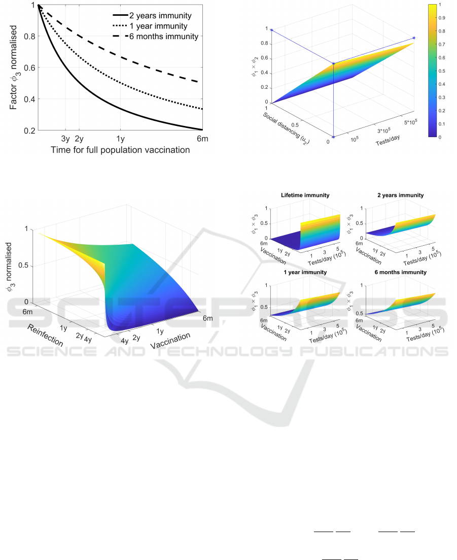
Figure 4: Contribution of u
6
, expressed as the expected time
to vaccinate all the population to φ
1
; three curves are re-
ported for different immunization times.
Figure 5: Dependence of φ
3
from vaccination and reinfec-
tion times.
A comparison between the contributions of the
controls to the reduction of R
u
, which can help in
the choice of type and intensity of the actions to ap-
ply, can be evidenced from Figures 6, 7 and 8; the
normalised reduction of the reproduction number is
reported under the action of two inputs at the same
time. From Figures 6 and 7 the low contribution of
the test campaign to the reduction of the spread can
be evidenced, at least with the rates considered. This
result is also contained in Figure 2, where a reduction
of R
u
(φ
1
) of less than 7%, under 6 · 10
5
tests/day, is
depicted.
Figures 6 and 8 show the sensible effect of a re-
duction of social contacts, as expected, strongly im-
proved by the combined action of vaccination (Figure
8). Unfortunately, a reduction of the benefits of vacci-
nation, under the hypothesis of a possible lost of im-
munity after a certain time, is well represented in Fig-
ures 7 and 8. In case of lifetime immunization, even a
quite low vaccination rate produces a strong contribu-
Figure 6: Combined effect of u
1
and u
2
to the spread reduc-
tion.
Figure 7: Combined effects of u
1
and u
6
to the spread re-
duction.
tion, only comparable with very high constraints on
social contacts. In presence of a limited time of im-
munization, the vaccination loses its great effective-
ness, becoming important its rate of execution with
respect to the one of reinfection.
In addition, it can be useful to study the contribu-
tion of the controls to the variation of the reproduction
number: it can represent an useful indication about
the most effective lines of intervention to produce a
larger variation of R
u
. One then can study the rela-
tive variation of R
u
w.r.t. the controls. Starting from
dR
u
=
∂R
u
∂φ
1
∂φ
1
∂u
1
du
1
+
∂R
u
∂φ
2
∂φ
2
∂u
2
du
2
+
∂R
u
∂φ
3
∂φ
1
∂u
6
du
6
(97)
Vaccination and Time Limited Immunization for SARS-CoV-2 Infection
617

Figure 8: Combined effects of u
2
and u
6
to the spread re-
duction.
and computing the three contributions
∂φ
1
∂u
1
= −φ
1

1
(u
1
+
m
1
a
)
+
1
(u
1
+
m
2
a
)

(98)
∂φ
2
∂u
2
= −β = −φ
2
1
1 − u
2
(99)
∂φ
3
∂u
6
= −φ
3
v
d
R
(ρ+d
R
)
(d
S
+ vu
6
d
R
(ρ+d
R
)
)
−φ
3
1
(d
S

1 +
ρ
d
R

+ vu
6
)
(100)
it is possible to write
dR
u
R
u
= −

1
(u
1
+
m
1
a
)
+
1
(u
1
+
m
2
a
)

du
1
−
du
2
1 − u
2
−
du
6
(d
S
(ρ+d
R
)
vd
R
+ u
6
)
(101)
The contribution of each control to the variation of
R
u
is depicted in Figures 9–11. The graphs confirm
the previous results: the test campaign contributes to a
limited reduction of the reproduction number of about
3.5 % almost independently from the rate of tests per-
formed, according to Figure 9. Differently, policies to
reduce the physical interactions between people have
a large impact on virus spread reduction, with an in-
creasing contribution as their intensity increase, as de-
picted in Figure 10 along with the particular of the
initial shape. It must be considered that u
2
= 1 corre-
sponds to the unrealistic total isolation of each person.
The opposite behaviour can be observed in Figure 11
for the vaccination: the higher is its rate, the smaller is
the relative reduction of R
u
; the reduction decreases
also in presence of reinfection and according to the
time of immunity presence.
Figure 9: Relative variation of R
u
due to changes of u
1
.
Figure 10: Relative variation of R
u
due to changes of u
2
.
6 CONCLUSIONS
In the present paper a model of COVID-19 is con-
sidered introducing also the vaccination as a control
input and, at the same time, the possibility of lost of
immunity, according to the present knowledge on the
Figure 11: Relative variation of R
u
due to changes of u
6
for
diffferent time of reinfection.
ICINCO 2021 - 18th International Conference on Informatics in Control, Automation and Robotics
618

effects of the available vaccines and the clinical evo-
lution of people previously infected and healed.
An analysis of steady state behaviour of the model
is performed, both in the classical uncontrolled case
and, in view of the subsequent study, under the hy-
pothesis of non zero constant control.
All the computations aimed at the determination
of an expression for the reproduction number under
constant control actions, to be used for analysing the
impact of the controls and the reinfection on the virus
spread.
Along with the expected result that social distanc-
ing measurements are effective actions, with an in-
creasing relative increment as the level of restriction
increases, the relative small contribution of the test
campaign is observed.
The new result obtained is related to the effect
of the vaccination on the epidemic containment and,
possibly, extinction. The high impact against the virus
spread is proved, but once the possibility that the im-
munization given by the vaccine has a limited dura-
tion is considered, the real effectiveness of the vac-
cine reduces, and depends on the rate of people vac-
cination with respect to the rate of immunity lost. On
the basis of the computation performed, if the time
of vaccination of the entire population is the same
as the immunity duration, the reproduction number
is halved w.r.t. its original value, despite intuitively
it could seem that, under the same rates, the popula-
tion should be, at steady state, completely vaccinated.
For a disease with R
0
' 3.6 as given for Italy, re-
duction factor must be smaller than
1
3.6
= 0.277: with
the vaccine as the only intervention measurement, a
vaccination rate four times the reinfection one is nec-
essary (Figure 4). An alternative solution could be
represented by keeping social restrictions at the min-
imum level for which an additional reduction factor
is present (Figures 3 and 8). These results suggest to
maintain socially acceptable but non null contact lim-
itations, even if infection trends are satisfactory, and
to speed up the vaccination until levels of immunised
individual is fully compatible with a herd immunity
status.
REFERENCES
Billah, M. A., Miah, M. M., and Khan, M. N. (2020).
Reproductive number of coronavirus: A systematic
review and meta-analysis based on global level evi-
dence. PLoS ONE, 5(11):1–17.
Daley, D. J. and Gani, J. (1999). Epidemic Modelling: An
Introduction. Cambridge Studies in Mathematical Bi-
ology. Cambridge University Press.
Di Giamberardino, P. and Iacoviello, D. (2021). Evaluation
of the effect of different policies in the containment of
epidemic spreads for the COVID-19 case. Biomedical
signal processing and control, 65(102325):1–15.
Di Giamberardino, P., Iacoviello, D., Albano, F., and
Frasca, F. (2020). Age based modelling of SARS-
CoV-2 contagion: The Italian case. 24
th
Int. Conf.
on System Theory, Control and Computing (ICSTCC),
pages 274–279.
Diekmann, O., Heesterbeek, J., and Roberts, M. (2010).
The construction of next-generation matrices for com-
partmental epidemic models. J R Soc Interface,
7(47):873–885.
Diekmann, O., Heesterbeek, J. A. P., and Metz, J. A. J.
(1990). On the definition and the computation of
the basic reproduction ratio R
0
in models for infec-
tious diseases in heterogeneous populations. Journal
of Mathematical Biology, 28:365–382.
Dietz, K. (1993). The estimation of the basic reproduc-
tion number for infectious diseases. Stat Methods Med
Res., 2(1):23–41.
Gumel, A., Iboia, E., Ngonghala, C., and Elbasha, E.
(2021). A primer on using mathematics to understand
covid-19 dynamics: Modeling, analysis and simula-
tions. Infect Dis Model., 6:148–168.
Katul, G. G., Mrad, A., Bonetti, S., Manoli, G., and Paro-
lari, A. J. (2020). Global convergence of covid-19 ba-
sic reproduction number and estimation from early-
time sir dynamics. PLoS ONE, 15(9):1–22.
Kermack, W. O. and McKendrick, A. G. (1927). A contri-
bution to the mathematical theory of epidemics. Proc.
Roy. Soc. Lond. A, 115(772):700–721.
Martcheva, M. (2015). An introduction to mathematical
epidemiology. Text in Appl. Math. 61, Springer.
Perasso, A. (2018). An introduction to the basic reproduc-
tion number in mathematical epidemiology. ESAIM:
ProcS, 62:123–138.
Tang, B., Wang, X., Li, Q., Bragazzi, N. L., Tang, S., Xiao,
Y., and Wu, J. (2020). Estimation of the transmission
risk of the 2019-nCoV and its implication for public
health interventions. J. of Clinical Medicine, 9(2).
van den Driessche, P. (2017). Reproduction numbers of
infectious disease models. Infectious Disease Mod-
elling, 2:288–303.
Zhao, S., Lin, Q., Musa, J. R. S. S., Yang, G., Wang, W.,
Lou, Y., Gao, D., Yang, L., He, D., and Wang, M. H.
(2020). Preliminary estimation of the basic repro-
duction number of novel coronavirus (2019-nCoV) in
China, from 2019 to 2020: A data-driven analysis in
the early phase of the outbreak. Int. J. of Infectious
Diseases, 92:214–217.
Vaccination and Time Limited Immunization for SARS-CoV-2 Infection
619