TC-CNN: Trajectory Compression based on Convolutional Neural

Network

Yulong Wang

1,2,3

, Jingwang Tang

1,3

and Zhe Jia

School of Computer Science (National Pilot Software Engineering School),

Beijing University of Post and Telecommunications, Beijing, China

Science and Technology on Communication Networks Laboratory, Shijiazhuang, China

State Key Laboratory of Networking and Switching Technology, Beijing, China

Keywords: Automatic Identification System, Trajectory Compression, Convolutional Neural Networks, Threshold.

Abstract: With the Automatic Identification System installed on more and more ships, people can collect a large number

of ship-running data, and the relevant maritime departments and shipping companies can also monitor the

running status of ships in real-time and schedule at any time. However, it is challenging to compress a large

number of ship trajectory data so as to reduce redundant information and save storage space. The existing

trajectory compression algorithms manage to find proper thresholds to achieve better compression effect,

which is labor-intensive. We propose a new trajectory compression algorithm which utilizes Convolutional

Neural Network to perform points classification, and then obtain a compressed trajectory by removing

redundant points according to points classification results, and finally reduce the compression error. Our

approach does not need to set the threshold manually. Experiments show that our approach outperforms

conventional trajectory compression algorithms in terms of average compression error and fitting degree

under the same compression rate, and has certain advantages in time efficiency.

1 INTRODUCTION

In recent years, with the continuous expansion of the

scale of global trade, shipping has gradually become

the main means of trade transportation among

countries. In order to ensure the safety of the marine

navigation vessel, position the vessel in real-time (G.

Pallotta, M. Vespe, and K. Bryan, 2013), plan the

channel for the management of maritime traffic, and

improve the efficiency of the ship (Al-Zaidi R, Woods

J. C., Al-Khalidi M., et al., 2018), the International

Maritime Organization demands that ships with more

than 300 tons must be equipped with Automatic

Identification System (AIS) (Muckell J., Hwang J. H.,

Lawson C. T., et al., 2010), through which a ship

sends its own position coordinates to nearby base

stations. The shore-based equipment can generate the

corresponding ship trajectory data based on these time

series containing the real-time coordinates of the ship.

However, due to the large number of ships, the daily

generated data will be huge, and there are a lot of

redundant data, which not only consume a great

amount of memory space, but also increase the burden

of server analysis and route data processing (Vries G.,

Someren M. V., 2012). Therefore, how to compress

the AIS trajectory data effectively has attracted many

researchers.

Trajectory compression algorithms are mainly

classified to offline algorithm and online algorithm.

This paper focuses on the offline trajectory

compression algorithm. An offline trajectory

compression algorithm obtains a complete original

track and then compresses it. Douglas Peucker

algorithm (DP) is the most classical offline

compression algorithm. It determines which points

need to be eliminated by recursive segmenting of

tracks, from whole to local, and gradually refining

compression interval (Liu J., Li H. & Yang Z., et al,

2019). Singh et al. (Singh A. K., Aggarwal V. &

Saxena P., et al., 2017) proposed a SPM algorithm

based on the DP algorithm. It adjusts the selection of

baseline of error measurement and compares the error

of trajectory points in turn using new error

measurement methods. Long et al. (Long Hao et al.,

2018) proposed a Trajectory Compression algorithm

170

Wang, Y., Tang, J. and Jia, Z.

TC-CNN: Trajectory Compression based on Convolutional Neural Network.

DOI: 10.5220/0010577801700176

In Proceedings of the 2nd International Conference on Deep Learning Theory and Applications (DeLTA 2021), pages 170-176

ISBN: 978-989-758-526-5

with Adaptive parameters (ATC), where the

automatic threshold calculation is realized by

inputting an expected compression rate λ by users.

Kangasuan et al. (Hansuddhisuntorn K., Horanont T.,

2019) proposed Improvement of TD-TR Algorithm.

Inspired by the success of deep learning in recent

years, this paper aims to improve the performance of

trajectory compressing by using Convolutional

Neural Network (CNN). A new algorithm, named

Trajectory Compression based on Convolutional

Neural network (TC-CNN) is proposed, which

utilizes CNN to perform points classification, and

then obtain a compressed trajectory by removing

redundant points according to points classification

results, and finally reduce the compression error. The

contributions of this paper are as follows:

1 To the best of our knowledge, it is the first work

to utilize deep learning technique on the problem

of offline trajectory compression. The CNN-

based recognition of feature points and non-

feature points is leveraged to compress tracks.

2 The designed CNN can classify the feature

points and redundant points in the track with

high precision, and significantly reduces the cost

of labour-intensive threshold adjustments

required by most of the existing trajectory

compression algorithms;

3 Experiments are conducted to compare the

performance of the proposed approach with

several benchmark algorithms. The results show

the efficacy of the proposed approach.

2 RELATED WORK

2.1 Trajectory Compression Algorithm

Douglas–Peucker (DP) (Singh A K, Aggarwal V &

Saxena P, 2017) is the most classic algorithm in the

off-line trajectory compression algorithm. It needs to

set a distance threshold

ε , and then calculate the

maximum vertical distance between the other points

in the track and the starting and ending points of the

track. If the distance is less than the threshold, then all

the points except the starting and ending points of the

track will be removed as redundant points. If the

distance is greater than the threshold, the trajectory is

split from the point, and then the sub trajectory is

recursively processed. DP is used widely as a

benchmark of trajectory compression algorithm.

Trajectory compression algorithm with adaptive

parameters (ATC) (Long Hao et al., 2018) abandoned

the compression threshold in the traditional trajectory

compression algorithm by setting the compression

ratio λ, and used the compression ratio to calculate the

threshold automatically. At the same time, the

compression algorithm is divided into three stages.

Firstly, the synchronous Euclidean distance of

each trajectory data point is calculated, and the

maximum value is selected.

Secondly, the compression threshold ε is

calculated according to the preset compression ratio λ

and the maximum synchronous Euclidean distance. If

the current Trajectory compression ratio is greater

than the preset value λ, the current Trajectory

compression threshold will be adjusted to 90% of the

previous compression threshold each time except for

the first time to achieve the purpose of automatic

calculation of the threshold until the compression

ratio is less than λ.

Finally, the first point whose synchronous

Euclidean distance is greater than ε will be found as

the dividing point. At the same time, all the track

points whose synchronous Euclidean distance is less

than ε will be eliminated. According to the dividing

point, the track composed of the remaining points will

be divided into two new tracks, and then the ATC

algorithm will be used recursively to compress until

the compression ratio is less than or equal to λ.

ATC achieves a relatively high fitting degree, but

incurs a low execution efficiency.

2.2 Trajectory Compression Evaluation

Metric

The widely used evaluation metric is Trajectory

Compression Ratio (TCR). The main purpose of

trajectory compression algorithm is to fit the original

trajectory with as few data points as possible, so as to

reduce the memory occupation of trajectory while

reducing the distortion of trajectory as much as

possible. Therefore, TCR is usually an important

metric for measuring the effectiveness of a trajectory

compression algorithm. TCR is defined as the

percentage of the number of track points P

after

compression and the number of track points P

before

compression, as shown in Eqn. (1)

(1)

Another metric is Average Compression Error

(ACE). It is the difference between the original track

and the compressed track in geometry. The

TC-CNN: Trajectory Compression based on Convolutional Neural Network

171

calculation of ACE is as follows. First, label the

original track in time order. Second, calculate the

vertical Euclidean error of each removed point in the

compressed track. Third, use the reserved point label

in the current track and its closest two points as the

reference point to calculate the vertical Euclidean

distance of the datum line. Finally, the sum of all

calculated values is divided by the number of original

trajectory points to obtain ACE. An ACE δ can be

calculated by Eqn. (2)：

()

，



,x,r

(2)

where m is the number of original trajectory points;

(i = 1, ..., n) is a removed point; The subscript i is the

label of the point in the original trajectory; x

and y

are the front and back points of

; d is the vertical

Euclidean distance between

and the line

determined by

and y

3 PROBLEM DEFINITION

In this section, the trajectory compression related

definitions are provided.

Define 1. Trajectory. The AIS data generated by a

ship on the sea can be regarded as a two-dimensional

coordinate point with time dimension and

geographical location dimension (T

). The line

segment formed by the same ship in order of time

coordinates is the ship's navigation track in a period

of time. The trajectory includes the location, time,

direction, route, and geographical area of the ship.

The two most important attributes are time and

geographical coordinates, so the ship's moving

trajectory can be regarded as a mapping relationship

from time to space M：T

→G

. Among them, M is a

continuous function based on time change, and its

independent variable time t belongs to Ti. Through

this function and a certain time value, a two-

dimensional coordinate corresponding to the ship at

this time point can be obtained(x

Define 2. Redundant Points and Feature Points. In

a track with multiple points, if some of them are

removed, only the remaining points can fit the

original track well, and the information loss is within

the acceptable range, the removed track points are

called redundant points, and the remaining points are

called feature points.

Define 3. Precursor Point and Successor Point.

Hypothesis p

is a point on the trajectory T = {p

i-2

, p

, ..., p

i+n

}, of the same ship in a continuous time series,

Then the two points adjacent to each other in the time

series are the adjacent points of the trajectory. The point

earlier than p

is called the precursor point of p

, and the

point later than p

is called the successor point of p

Definition 4. Synchronous Euclidean distance

(

Singh A K, Aggarwal V & Saxena P

, 2017). Hypothesis

is a point in the original trajectory，Connect the

starting and ending points of the datum of p

(which

can be the precursor and successor points of the point).

If the ship is regarded as moving at a constant speed

during this period, the distance between p

` and the

projection point p

` of its synchronous position on the

starting and ending line of the datum is its

synchronous Euclidean distance, which is greater than

or equal to the vertical distance from p

` to the starting

and ending line of the datum. As shown in Fig. 1.

Figure 1: Illustration of synchronous Euclidean distance.

The solid line segment is a track from point A to

point E, AE is the connecting line segment composed

of the datum starting and ending points A and E of G,

the perpendicular foot of point G on the AE

connecting line is point G, and the time interval

between A and G is t

, The time interval of AE is t

and AE can be regarded as a function of time interval

, Where 0

≤

, Then the coordinate point of

projection point C of G on AE should be

tt =

(3)

)(x

mnmi

x −×+=

(4)

)(y

i mnm

y −×+=

(5)

In AIS trajectory processing, in order to facilitate

practical use, improve calculation accuracy and

DeLTA 2021 - 2nd International Conference on Deep Learning Theory and Applications

172

reduce errors, the longitude and latitude coordinates

in AIS data are usually converted to their

corresponding Mercator coordinates (

Walkenhorst B T,

Nichols S

,2020). Eqn. (6-9) are used to calculate

Mercator coordinate, where

is the radius of the

datum latitude circle, a is the radius of the major axis

of the earth's ellipsoid, q is the equivalent dimension,

and e is the first eccentricity of the earth's ellipsoid (

Houpu, Li Haibo & Tang Qinghui

., 2019). Suppose that

the longitude and latitude coordinates of G are

),(

, and its corresponding Mercator coordinates

are (φ,ω).

ϕϕ

cossin1

×−

(6)

ϕϕπ

sin1

)

tan(ln

−

−+=

(7)

×=

(8)

qr ×=

(9)

Suppose that the coordinate of point G is

),,(

iii

tyx

. The coordinate of projection point C of

its synchronous position is

),,(

、、、

iii

tyx

. Then the

coordinate calculation of C is：

)(`x

−

−×

−

−+

−

(10)

)(`y

1 −+

−+

−

−×

−

(11)

From the Mercator coordinates (φ,ω) of G and the

Mercator coordinates (φ`,ω`) of the projection point

C of its synchronous position, the synchronous

Euclidean distance of G can be obtained by Eqn. (12).

)`()`(sed

iiii

ωωφφ

−+−=

(12)

Eqn. (12) is the length of the GC segment, as

shown in Fig. 1.

4 TC-CNN

The proposed approach TC-CNN consists of two part:

the point classification CNN and the trajectory

compression algorithm, which are elaborated as

follows.

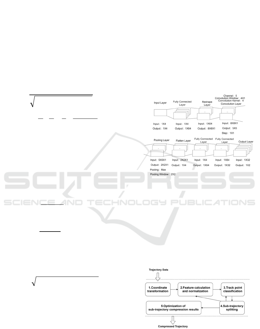
4.1 Point Classification CNN

We use an 8-layer CNN to classify the track points

into redundant points and feature points, whose

architecture is shown in Fig. 2. The input layer is

followed by a fully connected layer, and then a

flattening layer is connected to transform the input

into data with appropriate dimension. The third layer

is a convolution layer, which is followed by a max

pooling layer. After the data are reshaped by another

flatten layer, they are feed into two fully connected

layers one after another. Finally, the data are classified

by the output layer into two categories.

Figure 2: Architecture of the Point Classification CNN.

In the training phase the CNN, the epoch is 150,

the optimizer is Adam, the batch size is 64, the initial

learning rate is 0.005, and the cross entropy function

is used as the loss function.

4.2 Trajectory Compression Algorithm

The flowchart of the proposed trajectory compression

algorithm is shown in Fig. 3. The process of the

algorithm consists of five phases.

Figure 3: Flow chart of the proposed algorithm.

The first phase is coordinate transformation.

Because the coordinates of original trajectory data are

TC-CNN: Trajectory Compression based on Convolutional Neural Network

173

longitude and latitude coordinates, in order to ensure

the accuracy of feature calculation, it is necessary to

convert longitude and latitude coordinates into

Mercator coordinates.

The second phase is feature calculation and

normalization. For each point in the track, the

synchronous Euclidean distance of the corresponding

reference starting and ending points (i.e., the original

track or the split sub-track starting and ending points)

and the deflection angle, adjacent time difference and

adjacent speed difference based on the precursor point

and the successor point are calculated, respectively.

Then, the normalization operation is carried out, after

which the four features form a vector of features

corresponding to the trajectory point.

The third phase is track point classification. The

feature vector sequence corresponding to each point

of the original trajectory is input into the trained point

classification CNN, where each point is classified into

either redundant or feature points.

The fourth phase is sub-trajectory splitting. Based

on the output of the point classification CNN, the

original trajectories are divided into sub-trajectories

by using Alg. 1. The sub-trajectories are further

processed through the second and third phase. Then,

the redundant points in the sub-trajectories are

identified and removed.

The fifth phase is the optimization of sub-

trajectory compression results. According to the

classification results and Alg. 2, the compressed sub

trajectory is optimized, and the optimization results

are combined into a complete compression track.

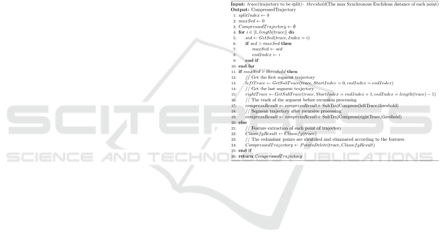
4.2.1 Sub-trajectory Compression

The feature of each point in a preprocessed original

trajectory T

= {t

, t

, …, t

} requires to be calculated.

Firstly, the synchronous Euclidean distance of the

rest points in the trajectory is calculated based on the

global view, with the starting point

and the ending

point t

as the reference points. At the same time, the

deflection angle, adjacent time difference and

adjacent speed difference are calculated based on the

precursor and successor points of each point

Secondly, the calculated feature sequence is input

into the trained network model for trajectory point

classification. The maximum synchronous Euclidean

distance of one or more trajectory points classified as

redundant points are used as the threshold, with which

the original track is split. The specific splitting

process is as follows: if the maximum synchronous

Euclidean distance of the track points except t

and t

is less than the threshold, the synchronous Euclidean

distance of other points in the sub-track is updated

with the starting and ending point of the current sub-

track as the reference point, and then the sub-track is

split. The trace is compressed. If the maximum

synchronous Euclidean distance of the point except t

and t

is greater than the threshold, the track is split

from the point.

Finally, the synchronous Euclidean distance of the

sub-trajectory is calculated with its start and

endpoints again.

The above process is carried out recursively, and

summarized as Alg. 1.

Algorithm 1: SubTrajCompress.

4.2.2 Compression Error Reduction

It is possible to further reduce the compression error

of the obtained trajectory.

Firstly, the data points in the original trajectory are

labeled according to their time order, and the intervals

are divided according to the trajectory splitting results

of Alg. 1.

Secondly, the original trajectory is divided into

optimized intervals according to the split sub

trajectory, and then the two trajectory points

belonging to different categories are replaced by

categories, so as to ensure that the compression ratio

will not be changed, After each transformation, the

average compression error and Hausdorff distance

between the current trajectory segment and the

original trajectory segment are calculated, and the

result with the smallest error is retained as the

optimization result of the current trajectory segment.

Finally, the optimized compressed trajectory can

be obtained by combining the optimization results of

DeLTA 2021 - 2nd International Conference on Deep Learning Theory and Applications

174

each trajectory segment.

The above process is summarized as Alg. 2.

Algorithm 2: ReduceCompressErr.

5 EXPERIMENTS

5.1 Data Set for CNN Training

The training data are from AIS records. The sample of

feature points and redundant points are obtained by

using several conventional trajectory compression

algorithms, e.g. SPM algorithm based on synchronous

Euclidean distance, improved top-down time ratio

compression algorithm, ATC algorithm based on an

adaptive threshold. In the end, we build a training data

set with 18,000 feature points and 18,000 redundant

points.

5.2 Experimental Results

In this section, the run time, TCR and ACE of TC-

CNN are evaluated and compared with the DP and

ATC. Due to the large amount of AIS data, only part

of the ship data is randomly selected as experimental

data to verify the algorithm model effect. In order to

ensure the preciseness of the experimental results, all

the experimental results are based on the compression

ratio of the proposed approach. The threshold or

compression ratio of the compared algorithms are

tuned to be close to each other with a variance of no

more than 2%. The database is MongoDB, the GPU

card is gtx1060ti, the memory is 16GB, the CPU is

3.4GHz Core i7 7700hq.

5.2.1 Comparison of Run Time and TCR

The time complexity of the considered algorithms are

all O(nlogn). In order to compare the actual time

performance of each algorithm, we use 1200 AIS

trajectories (including 1657647 data points) to test the

time cost of each algorithm under different

compression rates, and the results are shown in Table 1.

Table 1: Run Time under different TCR.

Algorithm

TCR

RunTime/ms

0.859

371,348.00

ATC

0.876

762,596.00

TC-CNN

0.872

621,574.00

It can be seen from table 1 that ATC algorithm has

the largest time cost, DP algorithm has the lowest time

cost, and TC-CNN algorithm is in between the time

cost of TC-CNN algorithm is higher than that of DP

algorithm because of the time consumption of data

preprocessing. If the ideal trajectory data is

compressed, the time performance cost of TC-CNN

algorithm will be close to that of DP algorithm.

Therefore, compared with the ATC algorithm, TC-

CNN algorithm has some advantages in running time.

5.2.2 Comparison of ACE

The author randomly selected 10, 50, 100, 200 and

500 ship trajectories from AIS actual data to carry out

the average compression error experiments

(compression rate ranges are [0.914,0.928],

[0.938,0.954], [0.851,0.869], [0.925,0.942],

[0.872,0.889]). The results are shown in Table 2.

Table 2: Comparison of ACE.

#traj. 10 50 100 200 500

DP 3.51 3.01 4.86 3.34 4.35

ATC 3.09 2.66 4.18 2.97 3.82

TC-CNN 3.18 2.47 3.64 2.85 3.23

As can be seen from Table 2, the average

compression error of DP algorithm is the highest. Due

to the introduction of synchronous Euclidean distance

to measure the time and space characteristics of the

trajectory, the compression error of ATC algorithm is

lower than that of DP algorithm. The average

TC-CNN: Trajectory Compression based on Convolutional Neural Network

175

compression error of TC-CNN algorithm is close to

that of ATC algorithm. Although the average

compression error of TC-CNN algorithm is slightly

higher than that of ATC algorithm when the number

of experimental samples is small (10 data), with the

increase of the number of experimental samples, the

average compression error of TC-CNN algorithm is

gradually lower than that of ATC algorithm.

Considering that there may be some specific

trajectories in the experiment of a small number of

data samples, which have better agreement with some

algorithms, the average compression error of TC-

CNN algorithm is higher than that of ATC algorithm

This part of the algorithm performs better, so a large

number of data sample experiments can better reflect

the overall effect of the algorithm, so on the whole,

the average compression error of TC-CNN algorithm

is the lowest. The results show that the accuracy of

TC-CNN algorithm is higher.

6 CONCLUSIONS

This paper proposes a trajectory compression

approach based on convolutional neural network

Trace compression algorithm can not only eliminate

the blindness of threshold determination, but also has

better applicability. It can improve the compression

accuracy of the network model by using a training set

with better feature differentiation or adding training

set data. The experimental results show that the

proposed approach can retain the key features of the

original trajectory and fit the original trajectory well,

and its compression effect is better than some

traditional offline trajectory compression algorithms.

But the algorithm still has some shortcomings, such

as the time cost is still large, in addition, how to obtain

typical data sets for model training, in order to

improve the accuracy of model compression results,

this is the direction of the next step.

ACKNOWLEDGEMENTS

This work is funded by Open Fund Project of Science

and Technology on Communication Networks

Laboratory (Grand No HHX21641X003)

REFERENCES

Pallotta, Giuliana, Vespe, et al. Vessel Pattern Knowledge

Discovery from AIS Data: A Framework for Anomaly

Detection and Route Prediction[J]. Entropy, 2013.

Al-Zaidi R., Woods J. C., Al-Khalidi M., et al. Building

Novel VHF-Based Wireless Sensor Networks for the

Internet of Marine Things[J]. IEEE Sensors Journal,

2018, 18(5):1-1.

Muckell J., Hwang J. H., Lawson C. T., et al. Algorithms for

compressing GPS trajectory data[C]// 2010:402.

Vries G., Someren M. V. Machine learning for vessel

trajectories using compression, alignments and domain

knowledge[J]. Expert Systems with Applications, 2012,

39(18):13426-13439.

Liu J., Li H., Yang Z., et al. Adaptive Douglas-Peucker

Algorithm with Automatic Thresholding for AIS-Based

Vessel Trajectory Compression[J]. IEEE Access, 2019,

7:150677-150692.

Singh A. K., Aggarwal V., Saxena P., et al. Performance

analysis of trajectory compression algorithms on marine

surveillance data[C]// 2017 International Conference on

Advances in Computing, Communications and

Informatics (ICACCI). 2017.

Long Hao, Zhang Shukui, Sun Penghui. Trajectory

compression algorithm with adaptive parameter,

Application Research of Computers[J], 2018, 35(3),

pp.685-688,716.

Hansuddhisuntorn K., Horanont T. Improvement of TD-TR

Algorithm for Simplifying GPS Trajectory Data[C]//

2019 First International Conference on Smart

Technology & Urban Development (STUD), 2019.

Walkenhorst B. T., Nichols S. Revisiting the Poincaré

Sphere as a Representation of Polarization State[C]//

2020 14th European Conference on Antennas and

Propagation (EuCAP), 2020.

Li Houpu, Li Haibo, Tang Qinghui, Direct transformation

between equiangular and equiarea, orthographic

cylindrical projections in the case of ellipsoid[J],

Journal of marine technology, 2019(5):15-20.

Douglas D. H., Peucker T. K., Algorithms for the Reduction

of the Number of Points Required to Represent a

Digitized Line or its caricature[J]. Canadian

Cartographer, 2006, 10(2):112-1.

DeLTA 2021 - 2nd International Conference on Deep Learning Theory and Applications

176