A Flexible Structured Solver for Continuous-time Algebraic Riccati
Equations
Vasile Sima
1,2 a
1
Modelling, Simulation, Optimization Department,
National Institute for Research & Development in Informatics,
Bd. Mares¸al Averescu, Nr. 8–10, Bucharest, Romania
2
Technical Sciences Academy of Romania, Romania
Keywords:
Balancing, Hamiltonian Matrix, Numerical Methods, Optimal Control, Riccati Equation.
Abstract:
The solution of algebraic Riccati equations (AREs) is a fundamental computation in optimal control and other
domains. The available solvers lack t he flexibility in choosing a solution technique, or specifying options and
parameters. The quality of a computed solution depends not only on the problem conditioning, but also on
the various decisions made by the solver designer. This paper proposes a flexible solver for continuous-time
AREs that allows the user to choose among several structured solution approaches, orthogonalization methods,
and balancing options and parameters. No selection ensures the best results for all problems. Therefore, it
is sometimes useful to try alternative pathways and find the best solution. The new solver has been used to
solve the examples from the SLICOT CAREX benchmark collection. The numerical results in extensive tests
illustrate the good performance of the proposed flexible solver.
1 INTRODUCTION
The solution of continuous-time and discrete-time al-
gebraic Riccati equations (CAREs and DAREs) is a
basic computation in control systems design, opti-
mal control and other domains. CAREs and DAREs
appear in many applications, such as, stabiliza-
tion and linear-quadratic regulator problems, Kalman
filtering, linear-quadratic Gaussian (LQG) optimal
control problems, computation of (sub)optimal H
∞
controllers, model reduction techniques based on
stochastic, positive or bounded real LQG balancing,
and factorization procedures for transfer functions.
Generalized CAREs and DAREs are given by the
following equations with unknown matrix X
Q + A
H
XE + E
H
XA
− (E
H
XB +L )R
−1
(B
H
XE + L
H
) = 0, (1)
Q + A
H
XA −E
H
XE
− (A
H
XB +L )(B
H
XB +R)
−1
(B
H
XA +L
H
) = 0,
(2)
where A,E,Q ∈ C
n×n
, B,L ∈ C
n×m
, R ∈ C
m×m
, C is
a
https://orcid.org/0000-0003-1445-345X
the complex plane, and the superscript H denotes the
complex conjugate. In the real case, H is replaced
by T , denoting the transposition operator. In appli-
cations, usually the stabilizing solution is required,
which can be used to stabilize the closed-loop sys-
tem matrix pencil. The assumptions made to ensure
that there is a unique stabilizing solution for each
equation above are that E is nonsingular, Q = Q
H
,
R = R
H
(with R nonsingular for (1)), and the Hamil-
tonian/symplectic pencil associated to (1)/(2) has no
eigenvalues on the imaginary axis/unit circle in C.
Sufficient conditions to guarantee the above assump-
tions are the stabilizability and detectability of the un-
derlying dynamical system, and the following positive
semidefiniteness property,

Q L
L
H
R

≥ 0. (3)
A very important class of CARE/DARE solvers
makes use of stable invariant or deflating subspaces
of some structured matrices or pencils. A matrix pen-
cil λS − H, with λ ∈ C, is Hamiltonian if HJS
H
=
−SJH
H
, and it is symplectic if HJH
H
= S JS
H
, where
J :=

0 I
n
−I
n
0

, J
T
= −J = J
−1
,
and I
n
denotes the identity matrix of order n. If S =
78
Sima, V.
A Flexible Structured Solver for Continuous-time Algebraic Riccati Equations.
DOI: 10.5220/0010577700780089
In Proceedings of the 18th International Conference on Informatics in Control, Automation and Robotics (ICINCO 2021), pages 78-89
ISBN: 978-989-758-522-7
Copyright
c
 2021 by SCITEPRESS – Science and Technology Publications, Lda. All rights reserved

I
2n
, definitions for Hamiltonian and symplectic ma-
trices are obtained; for instance, H is Hamiltonian if
(HJ)
H
= HJ; S is skew-Hamiltonian if (SJ)
H
= −SJ.
If the standard conditions mentioned above are
satisfied, and in addition, for DARE, A and R are non-
singular, the stabilizing solution of a CARE/DARE
can be obtained using an orthogonal basis of the sta-
ble invariant subspace of the Hamiltonian/symplectic
matrix (4)/(5),
H =

A − BR
−1
L
H
−BR
−1
B
H
−Q + LR
−1
L
H
LR
−1
B
H
− A
H

, (4)
H =

e
A + BR
−1
B
H
e
A
−H
e
Q −BR
−1
B
H
e
A
−H
−
e
A
−H
e
Q
e
A
−H

, (5)
where
e
A := A − BR
−1
L
H
,
e
Q := Q − LR
−1
L
H
.
The explicit need of matrix inversion in the
CARE/DARE solvers using (4)/(5) (for instance, of
matrix A, for symplectic DARE solvers) can ruin the
accuracy of the results, if the matrix to be inverted
is ill-conditioned. Better results can be obtained us-
ing stable deflating subspaces of extended matrix pen-
cils, with no inversion involved (see, e.g., (Bender
and Laub, 1987a; Bender and Laub, 1987b; Lancaster
and Rodman, 1995; Mehrmann, 1991; Sima, 1996;
Van Dooren, 1981)) for CAREs and DAREs:
H =


A 0 B
Q A
H
L
L
H
B
H
R


, S =


E 0 0
0 −E
H
0
0 0 0


, (6)
H =


A 0 B
Q −E
H
L
L
H
0 R


, S =


E 0 0
0 −A
H
0
0 −B
H
0


, (7)
respectively. The solvers available, e.g., in
MATLAB
®
Control System Toolbox (MathWorks
®
,
2015) and SLICOT (Benner et al., 1999; Benner et al.,
2010), are using the standard QZ algorithm for re-
ordering the eigenvalues, to determine the stable de-
flating subspaces. The special structure of the matrix
pencils involved is not exploited.
Recently, structure-exploiting techniques have
been investigated for solving Hamiltonian and skew-
Hamiltonian/Hamiltonian eigenproblems, see, e.g.,
(Benner et al., 2002; Benner et al., 2007), and the ref-
erences therein. These techniques can be employed
for CARE solvers. For solving DAREs, it is possible
to preprocess the pencils by an extended Cayley trans-
formation, which only involves matrix additions and
subtractions (Xu, 2006), to obtain equivalent skew-
Hamiltonian/Hamiltonian pencils. However, matrix
inversions are still needed for DAREs.
This paper addresses the real continuous-time
AREs using structured eigensolvers. Important ingre-
dients are the reduction to condensed forms, such as
(generalized) symplectic URV decomposition (Ben-
ner et al., 1997; Benner et al., 1998), structured
Schur form (Benner et al., 2007; Benner et al.,
2016), and periodic Schur decomposition (Bojanczyk
et al., 1992; Sreedhar and Van Dooren, 1994; Granat
et al., 2007a; Granat et al., 2007b). A new, flex-
ible solver, scare , has been developed based on
SLICOT Library routines (Benner et al., 1999; Ben-
ner et al., 2010) and the associated MATLAB M-
and MEX-files. It uses the latest version of the pe-
riodic QZ solver discussed in (Sima, 2019; Sima and
Gahinet, 2019; Sima and Gahinet, 2020), and of the
balancing techniques for Hamiltonian matrices and
skew-Hamiltonian/Hamiltonian matrix pencils (Ben-
ner, 2001; Sima, 2016; Sima and Benner, 2016). Sev-
eral approaches are implemented, and the solver can
select one automatically, or it can try to use a speci-
fied one. The new solver has been used to solve the
CARE examples from SLICOT CAREX benchmark
collection (Abels and Benner, 1999). The previous
results (Benner and Sima, 2003; Benner et al., 2016;
Sima, 2011) have been improved. Since no algo-
rithm or set of fixed options and parameters are guar-
anteed to obtain the best performance for all prob-
lems,
scare has been invoked successively with all
approaches and several balancing options and related
parameters. The best results in terms of relative errors
and relative residuals have been found automatically
by calling MATLAB MEX-functions in a loop.
Besides the development of the new solver and of
some improvements of the invoked periodic QZ and
skew-Hamiltonian/Hamiltonian procedures, as well
as of the related balancing, our contributions include
the design and realization of the tools for exploring
the solver capabilities over the range of available op-
tions and parameter values. This enables to find im-
proved solutions in terms of relative errors (to known
or reference solutions) and relative residuals, and to
assess the solver performance and make extensive
comparisons with state-of-the-art MATLAB solvers.
2 STRUCTURED APPROACHES
FOR THE CARE SOLVER
The quality of a computed solution depends on the
conditioning of the equation or problem itself, but
also on the method used by the solver and on the avail-
able parameters and/or options. The scare solver
uses two main structured solution approaches: Hamil-
tonian approach and skew-Hamiltonian/Hamiltonian
A Flexible Structured Solver for Continuous-time Algebraic Riccati Equations
79

approach, but also a derived one, Hamiltonian pencil
approach.
The Hamiltonian approach can be applied if the
matrix E is identity, E = I
n
, and the matrix R is well-
conditioned. This approach operates on the matrix,
obtained from (4),
H =

A −
e
BD
−1
e
L
T
−
e
BD
−1
e
B
T
−Q +
e
LD
−1
e
L
T
e
LD
−1
e
B
T
− A
T

, (8)
where
e
B := BU ,
e
L := LU, U and D are the factors of
a Schur decomposition of the matrix R, R = UDU
T
,
with U orthogonal, and D diagonal. (If R is diag-
onal, then D = R and U = I
m
.) The Schur decom-
position also enables to reliably asses the numerical
conditioning of R, since its condition number is κ :=
max(|D|)/min(|D|), where max(|D|) and min(|D|)
denote the maximum and minimum absolute value
of the diagonal elements of D; note that min(|D|)
is theoretically nonzero, since R is assumed nonsin-
gular. Usually, R is considered well-conditioned if
κ < 1/ε
1/2
, where ε is the relative machine accu-
racy. Note that the matrix H in (8) is Hamiltonian,
since H
22
= −H
T
11
, H
12
= H
T
12
, and H
21
= H
T
21
, that
is, (HJ)
T
= HJ, where H
i j
∈ R
n×n
denotes the (i, j)
block of H.
The requirement on the well-conditioning of R is
needed in order to avoid inaccurate computations of
the H
i j
blocks of H, i, j = 1 : 2. (A MATLAB-style
notation for array indexing (MathWorks
®
, 2016) is
used.) In such a case, the Hamiltonian approach is
theoretically equivalent to a special case of the skew-
Hamiltonian/Hamiltonian approach, called Hamilto-
nian pencil approach, for convenience. The Hamilto-
nian pencil is defined by λS − H, where S = I
2n
, and
H is defined in (8). The matrix S is a special case
of a skew-Hamiltonian matrix, since S
22
= S
T
11
, S
12
=
−S
T
12
, and S
21
= −S
T
21
, that is, (SJ)
T
= −SJ. Note
that the numerical results obtained using the Hamilto-
nian matrix and Hamiltonian pencil approaches may
(slightly) differ.
The formula for H in (8) cannot be used if E is
not an identity matrix. In such a case, a more general
skew-Hamiltonian/Hamiltonian (pencil) approach is
used, with the matrices H and S defined starting
from (6). Since a skew-Hamiltonian/Hamiltonian
pencil must have an even size, k ≥ 0 fictitious control
inputs are added so that m + k is even. The optimal
problem for B and R replaced by

B
e
B

and block-
diag( R,
e
R ), respectively, with
e
B = 0 ∈ R
n×k
, and
e
R = I
k
has the same solution as the original problem.
The most convenient values are k = 0, if m is even,
and k = 1, otherwise. The extended matrices H and S
are defined below (see, e.g., (Sima, 2010) for details)
H =




A B
1
0 B
2
L
T
2
R
T
12
B
T
2
R
22
−Q −L
1
−A
T
−L
2
−L
T
1
−R
11
−B
T
1
−R
12




,
S =



E 0 0 0
0 0 0 0
0 0 E
T
0
0 0 0 0



, (9)
where B
i
∈ R
n×p
, L
i
∈ R
n×p
, R
i j
∈ R
p×p
, i, j = 1 : 2,
with p = (m + k)/2 and

B
1
B
2

:=

B
e
B

,


Q L
1
L
2
L
T
1
R
11
R
12
L
T
2
R
21
R
22


:=


Q L 0
L
T
R 0
0 0
e
R


.
(10)
It is easy to check that H is a Hamiltonian matrix
and S is a skew-Hamiltonian matrix. The matrix pen-
cil λS − H in (9) has the order 2
e
n, with
e
n := n + p.
Note that this extension will add 2p infinite eigen-
values; the solver has to be able to recognize and
remove these eigenvalues, since the original opti-
mization problem has 2n eigenvalues, and the sta-
ble deflating subspace should have n basis vectors.
Again, although the Hamiltonian pencil approach and
the skew-Hamiltonian/Hamiltonian approach theoret-
ically deliver the same solution if E = I
n
, the solutions
computed numerically may differ.
The automatic selection of the approach is based
on several rules and the default values of the option
parameters sHHpen and Hpen . Each of these parame-
ters may be set to logical values of true or false , but
the default is false . If sHHpen is false , E = I
n
, and
R is a diagonal matrix, or its condition number satis-
fies κ < 1/ε
1/2
, the Hamiltonian approach is automat-
ically selected. If the first two conditions above hold,
but R is ill-conditioned (κ ≥ 1/ε
1/2
), then the solver
resets internally sHHpen to true , enforcing the skew-
Hamiltonian/Hamiltonian pencil approach. The other
parameters (balancing option, threshold value for bal-
ancing, if requested, orthogonalization method) also
have default values. However, as stated before, better
results can sometimes be obtained with parameter val-
ues different than their default counterparts. There-
fore, the solver allows to specify the desired values,
but overrides inappropriate selections. For instance,
if sHHpen and Hpen are both set to true (that would
normally imply the selection of the Hamiltonian pen-
cil approach), but E is not an identity matrix, then the
skew-Hamiltonian/Hamiltonian pencil approach is in-
voked by resetting Hpen to false . The possibility to
specify the approach and related options and parame-
ICINCO 2021 - 18th International Conference on Informatics in Control, Automation and Robotics
80

ters increases the solver flexibility and enables to per-
form extensive tests and comparisons.
The essential computations for the three structured
approaches discussed above are the same. The first
step is the initial reduction of a double size embed-
ded matrix (pencil) to the (generalized) symplectic
URV decomposition using orthogonal symplectic ma-
trices and, then, to a (formal) matrix product in peri-
odic quasi-triangular form; in the pencil case, three
matrices (or five, if the initial S is J-semidefinite,
e.g., it is factored as S = JZ
T
J
T
Z) are upper trian-
gular, and another matrix is quasi-triangular, i.e., it
is block upper triangular with 1 × 1 and 2 × 2 diago-
nal blocks. Then, the periodic QZ algorithm is used
to reduce the matrix product to the periodic Schur
form, in which all 2 × 2 diagonal blocks correspond
to complex conjugate eigenvalues. Half of the fac-
tors are matrix inverses, which can be singular, but
the algorithm can deal with singularities. The next
step is to reorder the eigenvalues so that the stable
ones are moved to the leading positions of the ma-
trix product. The right transformations performed are
multiplied, and the first n columns of the result define
an orthogonal basis of the stable invariant or deflating
subspace of the matrix or matrix pencil, respectively.
If U is a basis matrix, and U
1
=U
1:n,:
, U
2
=U
˜n+1: ˜n+n,:
,
then the solution of the Riccati equation is given by
X = U
2
U
−1
1
, where U
1
is theoretically guaranteed to
be nonsingular under the assumptions in Section 1.
3 STRUCTURED BALANCING
FOR THE CARE SOLVER
Quite often, the matrices H (and S, for the pencil case)
have large norms and elements with highly different
magnitude. An example will be discussed in Sec-
tion 4. Other even more highlighting examples are
given in (Sima, 2016). Such matrices or matrix pen-
cils imply potential numerical difficulties for comput-
ing the eigenvalues and the invariant or deflating sub-
spaces, with negative consequences on the reliability
and accuracy of the results, see, e.g., (Sima and Ben-
ner, 2015a). Balancing procedures can be used to im-
prove the numerical behavior.
Balancing is intended to reduce the norms of
the given matrices and reduce the condition num-
ber of the problem, but this may not always be
achieved. Ward (1981) proposed a balancing tech-
nique for general matrix pencils, which has been in-
corporated in state-of-the-art software packages, such
as LAPACK (Anderson et al., 1999). (This will be re-
ferred below as standard balancing.) The data matri-
ces are preprocessed by equivalence transformations,
in two optional stages: the first stage uses permu-
tations to find isolated eigenvalues (which are avail-
able by inspection, with no rounding errors), and the
second stage uses diagonal scaling transformations to
make the row and corresponding column 1-norms as
close as possible. For general matrices or matrix pen-
cils, the first stage reshapes them so that the leading
and/or trailing parts are upper triangular, if possible.
In such a case, the eigenvalues corresponding to these
parts are readily available and perfectly accurate.
Balancing may reduce the 1-norm of the
scaled matrices, but this is not guaranteed.
Structure-preserving balancing techniques for
(skew-)Hamiltonian matrices and skew-Hamiltoni-
an/Hamiltonian matrix pencils have been developed
in (Benner, 2001) and (Sima, 2016), respectively.
These techniques first isolate, if possible, eigenvalues
in the elements 1 : ℓ − 1 and
e
n + 1 :
e
n + ℓ − 1 on
the diagonals of H, or of S and H, respectively;
this means that the columns 1 : ℓ − 1 are in an
upper triangular form, and the rows and columns
e
n + 1 :
e
n + ℓ − 1 are in a lower triangular form.
Then, diagonal equivalence transformations to the
rows and columns ℓ :
e
n and
e
n + ℓ : 2
e
n are applied,
to make the rows and corresponding columns as
close in 1-norm as possible. Due to the structure,
it is enough to equilibrate the 1-norms of the rows
and columns ℓ :
e
n of H (or S and H). But in order
to preserve the structure, all tranformations must be
symplectic for Hamiltonian matrices (Benner, 2001).
It is not always possible to keep the structure of H
(or of S and H) using only symplectic permutations,
P = block-diag(P,P), with P
T
P = I
n
, but generalized
symplectic permutations, which may also have values
set to −1 instead of 1, may be required.
For skew-Hamiltonian/Hamiltonian pencils it is
not necessary that all scaling transformations be sym-
plectic (Sima, 2016). For convenience, assume that
ℓ = 0. Let L and R be the left and right trans-
formations applied to S and H for balancing. If
L = block-diag(D
1
,D
2
), with diagonal matrices D
i
∈
R
˜n× ˜n
, i = 1 : 2, then R = block-diag(D
2
,D
1
). The
structure of S and H is preserved under these transfor-
mations. For ℓ > 0, the first ℓ − 1 diagonal elements
of D
1
and D
2
will be 1.
After solving an ARE using the skew-Hamilto-
nian/Hamiltonian approach applied to the balanced
pencil, λ
e
S −
e
H, the solution of the original prob-
lem must be recovered using inverse balancing. Let
e
U =
h
e
U
T
1
e
U
T
2

T
be a basis of the stable right deflating
subspace of λ
e
S −
e
H. When
e
n = n, the stabilizing so-
lution of the balanced ARE is given by
e
X =
e
U
2
e
U
−1
1
.
Since
e
U is related to a basis, U, of the stable right de-
A Flexible Structured Solver for Continuous-time Algebraic Riccati Equations
81

flating subspace of the original pencil, λS − H, by the
transformation
e
U = block-diag(D
−1
2
,D
−1
1
)U, it fol-
lows that

U
T
1
U
T
2

T
:= U = block-diag(D
2
,D
1
)
e
U.
Therefore, the stabilizing solution of the original ARE
can be computed as follows
X = U
2
U
−1
1
= D
1
e
U
2
e
U
−1
1
D
−1
2
. (11)
Formula (11) allows to represent and use the solution
X in a factored form, which may be useful for numeri-
cal reasons. When
e
n = n + p, with p > 0, only the first
n rows of U
1
, U
2
,
e
U
1
,
e
U
2
, D
1
, and D
2
will be used.
The balancing procedure is improved for enabling
to get meaningful results when standard balancing
(possibly even a structured variant) fails, see (Sima,
2016) for some numerical examples. An enhance-
ment of the iterative LAPACK balancing procedure
is used for finding the scaling factors, optionally lim-
iting their range via an outer loop. Specifically, a
threshold value, τ, can be set as an input argument. If
τ ≥ 0, the entries whose absolute values are smaller
than τM
0
, where M
0
= max(∥H(s, s)∥
1
,∥S (s, s)∥
1
),
with s := ℓ :
e
n ∪
e
n+ℓ : 2
e
n, are not considered for com-
puting the scaling factors.
If τ < 0 on entry, an outer loop over a sequence
of values τ
i
> 0 will select a set of scaling factors
which, if possible, will ensure the reduction of a de-
sired norm-related measure for the scaled matrices.
For τ = −1, this measure is the minimum of
max
i
(∥H
i
(s,s)∥
1
/∥S
i
(s,s)∥
1
,∥S
i
(s,s)∥
1
/∥H
i
(s,s)∥
1
),
where H
i
(s,s) and S
i
(s,s) are the scaled submatrices
corresponding to the threshold τ
i
. This strategy tries
to balance H and S, but also to make their 1-norms
comparable.
For τ = −2, the same measure is used, but if
max(∥
e
H(s,s)∥
1
,∥
e
S(s,s)∥
1
) > cM
0
and t > T , where
c and T are given constants (c possibly larger than
1), and t is the maximum ratio of the scaling factors
found (the maximum of the condition numbers of D
1
and D
2
), then the scaling factors are set to 1; here,
the matrices with tilde accent are the solution of the
above norm ratio reduction problem. This approach
avoids to obtain scaled matrices with too large norms,
compared to the given ones, and also limits the range
of the scaling factors.
For τ = −3, the measure used is the smallest prod-
uct of norms, min
i
(∥H
i
(s,s)∥
1
∥S
i
(s,s)∥
1
), over the
sequence of τ
i
values tried, while for τ = −4, the con-
dition numbers of the scaling transformations are ad-
ditionally supervised, and the scaling factors are set
to 1 if the “optimal” scaling has a condition number
larger than T . This tends to reduce the 1-norms of
both matrices.
Finally, if τ = −10
k
, the condition numbers of the
acceptable scaling matrices are bounded by 10
k
.
4 NUMERICAL RESULTS
The examples from the SLICOT CAREX benchmark
collection (Abels and Benner, 1999) have been used
to evaluate the performance of the implemented, flex-
ible solver, scare . All examples have been con-
sidered, with the parameters specified in (Abels and
Benner, 1999), except for Example 4.4, for which a
smaller size, namely N = 151, has been chosen, while
the default size in the cited reference is N = 211. (The
order of the system for this example is n = 2N − 1.)
For the default size, Example 4.4 is difficult for
any Riccati solver. Besides its large order, the asso-
ciated Hamiltonian matrix has a norm of over 4 · 10
11
and the magnitude of its elements is between 3· 10
−24
and 3.4 · 10
11
; the usual LAPACK-style scaling pro-
cedures even increase the norm and produce unusable
scaling factors and scaled matrices. Using a scaling
procedure similar to arescale in MATLAB R2015b,
the norm and the range of the element values have
been reduced by about six and eleven orders of mag-
nitude, respectively. But the computed solution may
still be inaccurate due to the occurrence of Hamilto-
nian eigenvalues near the stability boundary.
For convenience, the CAREX examples are num-
bered here from 1 to 34; they belong to four groups:
parameter-free problems of fixed size (examples 1–
6), parameter-dependent problems of fixed size (ex-
amples 7–24), scalable size problems without pa-
rameters (examples 25–28), and parameter-dependent
problems of scalable size (examples 29–34). Table II
in (Benner et al., 2016) lists the sizes and parameters
used for these 34 examples, together with the relative
residuals for the versions of the MATLAB function
care and skew-Hamiltonian/Hamiltonian solver then
available. This paper includes more and better results,
obtained using the new solver scare , that provides
higher flexibility and more options.
Two measures are used to assess the quality of
the computed solutions: the relative error and relative
residual. The relative error is defined by
∥X − X
∗
∥/max{1, ∥X
∗
∥}, (12)
where the 2-norm is used, X denotes the computed
solution, and X
∗
is the exact solution, if known, and
the solution returned by the MATLAB function care ,
otherwise. The exact solution is known for CAREX
examples 1.1, 1.2, 2.1.1-2, 2.3.1-3, 2.4.1-2, 2.5.1-2,
ICINCO 2021 - 18th International Conference on Informatics in Control, Automation and Robotics
82

2.6.1-2, 3.2.1-2, or, with renumbering, for examples
1, 2, 7, 8, 11 : 19, 27, and 28. (A notation like 2.1.1-
2 denotes the two examples 2.1, an easy one, and a
difficult one.) To allow a fair comparison, the relative
residual is defined as in care , namely,
∥T
1
− T
2
+ Q∥
1
/(1 + ∥T
1
∥
1
+ ∥T
2
∥
1
+ ∥Q∥
1
), (13)
where ∥ · ∥
1
refers to the 1-norm of the matrix ·, and
T
1
:= A
T
XE + E
T
XA,
T
2
:= (E
T
XB + L)R
−1
(B
T
XE + L
T
). (14)
The experiments have been performed on an Intel
Core i7-3820QM portable computer (2.7 GHz, 16 GB
RAM, relative machine precision ε
M
≈ 2.22 ×10
−16
),
using Windows 7 Professional (Service Pack 1) op-
erating system (64 bit), Intel Visual Fortran Com-
poser XE 2015 and MATLAB 6.0.267246 (R2015b).
The executables have been built using the MATLAB-
provided optimized LAPACK and BLAS subrou-
tines. Part of the tests have also been done with
MATLAB 9.9.0.1538559 (R2020b), Update 3. The
results obtained with this release are presented in the
figures having “(R2020b)” in their caption and title.
For each CAREX example, scare has been
called for each of the three approaches, if possi-
ble. (Example 2.2.2 has been solved using skew-
Hamiltonian/Hamiltonian approach, since the matrix
R has a large condition number, κ ≈ 4 · 10
−8
.) For
each pencil approach, three orthogonalization meth-
ods have been tried: QR factorization; QR factoriza-
tion with column pivoting; and singular value decom-
position (SVD). For each approach and method, the
following balancing options have been used: no bal-
ancing; row and column permutations; row and col-
umn scaling; row and column permutations and scal-
ing; balancing using an adaptation of the MATLAB
function arescale . For the pencil approaches, the
set of threshold values tried has been
τ ∈ {−10
3
,−10
2
,−10, −4 : 1 : −1,10ε, 10
2
ε,10
3
ε}.
The best results for all the trials and each example
have been recorded and processed. The results are
summarized below, and are better than those reported
in previous works, e.g., (Sima, 2011; Sima and Ben-
ner, 2015b).
Figure 1 shows the relative errors for examples
with known solutions from the CAREX collection,
using MATLAB function care and scare solver,
with the best options. Except for the fourth exam-
ple in the figure (i.e., example 2.1.2, for which the
pair (A,B) is almost unstabilizable), scare obtained
smaller relative errors than care . For this exam-
ple, care solution has an exceptionally small error,
of the order of 10
−29
. This is not the case for the
0 5 10 15
Example #
10
-30
10
-25
10
-20
10
-15
10
-10
10
-5
10
0
Relative errors
Relative errors for CAREX examples with known solution
scare
care
Figure 1: Relative errors for examples with known solu-
tions from the CAREX collection, using MATLAB function
care and scare solver, with the best options.
0 5 10 15
Example #
10
-20
10
-15
10
-10
10
-5
10
0
Relative errors
Relative errors for CAREX examples with known solution (R2020b)
scare
care
Figure 2: Relative errors for examples with known solu-
tions from the CAREX collection, using MATLAB function
care and scare solver, with the best options (MATLAB
R2020b).
MATLAB R2020b Release (see Fig. 2), when the rel-
ative error exceeded 10
−5
. (The other results with the
two releases are comparable.) Moreover, the relative
error of the scare solution for this numerically dif-
ficult example is quite good, namely 3.2751 · 10
−13
,
which is only three orders of magnitude bigger than
the machine accuracy. On the other hand, scare
shows improvements of six, five, and two orders of
magnitude for one, two, and two examples, respec-
tively.
Figure 3 plots the relative errors obtained by
scare , taking the care solutions as reference when
the true solution is not known. All examples from the
CAREX collection are considered. Only five exam-
ples (19, 23, 29, 30, and 34) have relative errors larger
than 10
−10
. Figure 4 presents similarly the results for
the MATLAB R2020b Release.
Figure 5 displays the relative residuals obtained
for scare and care for all examples. For three exam-
ples (8, 15, and 34, alias 2.1.2, 2.4.2, and 4.4), care
produced smaller relative residuals than scare , but
A Flexible Structured Solver for Continuous-time Algebraic Riccati Equations
83

0 5 10 15 20 25 30 35
Example #
10
-25
10
-20
10
-15
10
-10
10
-5
10
0
Relative errors
Relative errors for CAREX examples
scare
Figure 3: Relative errors for all examples from the CAREX
collection, using scare solver, with the best options; care
solution is used as reference when true solution is unknown.
0 5 10 15 20 25 30 35
Example #
10
-20
10
-15
10
-10
10
-5
10
0
Relative errors
Relative errors for CAREX examples (R2020b)
scare
Figure 4: Relative errors for all examples from the CAREX
collection, using scare solver, with the best options; care
solution is used as a reference when the true solution is not
known (MATLAB R2020b).
0 5 10 15 20 25 30 35
Example #
10
-18
10
-16
10
-14
10
-12
10
-10
10
-8
10
-6
10
-4
Relative residuals
Relative residuals for CAREX examples
scare
care
Figure 5: Relative residuals for examples from the CAREX
collection, using MATLAB function care and scare
solver, with the best options.
a big difference is only for example 2.1.2. See the
short discussion related to this example in the para-
graph presenting Fig. 1. On the other hand,
scare
shows improvements of four, three, two, and one or-
0 5 10 15 20 25 30 35
Example #
10
-18
10
-16
10
-14
10
-12
10
-10
Relative residuals
Relative residuals for CAREX examples with small values
scare
care
Figure 6: Relative residuals smaller than 10
−10
for exam-
ples from the CAREX collection, using MATLAB function
care and scare solver, with the best options.
0 5 10 15 20 25 30 35
Example #
10
-18
10
-16
10
-14
10
-12
10
-10
10
-8
10
-6
10
-4
Relative residuals
Relative residuals for CAREX examples (MATLAB R2020b)
scare
care
Figure 7: Relative residuals for examples from the CAREX
collection, using MATLAB function care and scare
solver, with the best options (MATLAB R2020b).
ders of magnitude for one, one, five, and two exam-
ples, respectively. The differences between the two
solvers are better seen in Fig. 6, which shows the re-
sults for examples for which the residuals are smaller
than 10
−10
.
Figure 7 plots the relative residuals for the
CAREX examples using MATLAB R2020b Re-
lease. The relative residuals are smaller for some
examples, but larger for other examples than for
MATLAB R2015b Release. Figure 8 shows the per-
formance for examples having the relative residu-
als for scare smaller than 10
−12
. Surprinsingly,
for more examples in Fig. 8, care obtained signifi-
cantly larger residuals than scare in comparison to
MATLAB R2015b (see Fig. 6). In particular, the rela-
tive residual for example 2.1.2 is over seven orders of
magnitude bigger for care than for scare .
Often, the minimum relative error for an exam-
ple is not obtained for the selection of options giving
the minimum residual. Figure 9 compares the best
relative errors for the CAREX examples with those
corresponding to the smallest relative residual. The
ICINCO 2021 - 18th International Conference on Informatics in Control, Automation and Robotics
84

0 5 10 15 20 25 30 35
Example #
10
-18
10
-16
10
-14
10
-12
10
-10
10
-8
10
-6
10
-4
Relative residuals
Relative residuals for CAREX examples with small values (MATLAB R2020b)
scare
care
Figure 8: Relative residuals smaller than 10
−12
(for scare )
for examples from the CAREX collection, using MATLAB
function care and scare solver, with the best options
(MATLAB R2020b).
0 5 10 15 20 25 30 35
Example #
10
-25
10
-20
10
-15
10
-10
10
-5
10
0
Relative errors
Relative errors for CAREX examples
scare
scare (error for minimum residual index)
Figure 9: Comparison of the best relative errors for scare
solver with the relative errors corresponding to the selection
of options giving the smallest relative residuals for exam-
ples from the CAREX collection.
0 5 10 15 20 25 30 35
Example #
10
-18
10
-16
10
-14
10
-12
10
-10
10
-8
10
-6
10
-4
Relative residuals
Relative residuals for CAREX examples
scare
scare (residual for minimum error index)
Figure 10: Comparison of the best relative residuals for
scare solver with the relative residuals corresponding to
the selection of options giving the smallest relative errors
for examples from the CAREX collection.
differences are not large, except for the examples 15
and 17, alias 2.4.2 and 2.5.2. The difference exceeds
five orders of magnitude for Example 2.4.2. Simi-
0 5 10 15
Example #
10
-20
10
-15
10
-10
10
-5
10
0
Relative errors
Relative errors for CAREX examples with known solution (balanc = 0)
scare
care
Figure 11: Relative errors for examples from the CAREX
collection with known solution using MATLAB function
care and scare solver with the best options, but without
balancing.
0 5 10 15 20 25 30 35
Example #
10
-20
10
-15
10
-10
10
-5
10
0
Relative errors
Relative errors for CAREX examples (balanc = 0)
scare
Figure 12: Relative errors for examples from the CAREX
collection using scare solver with the best options, but
without balancing;
care solution is used as a reference.
larly, Fig. 10 compares the best relative residuals with
those corresponding to the selection of options giv-
ing the smallest relative error. The largest differences
are for the examples 13, 30, 31, and 32 (2.3.3, 4.1.2,
4.2.1-2), with over four orders of magnitude for 13.
Figure 11 displays the relative errors for CAREX
examples with known solution using care and scare
with the best options, but without balancing. The er-
rors are usually comparable, but the differences ex-
ceed two and one order of magnitude for examples
2.1.2 and 2.3.2, respectively. Comparing these errors
with the smallest ones, obtained using balancing (see
Fig. 1), the advantage of balancing for badly scaled
or ill-conditioned examples is clear: the error is re-
duced by over 11, 6, 5, 5, 4, and 2 orders of magni-
tude for the examples 2.3.3, 2.1.2, 2.3.2, 2.4.2, 2.5.2,
and 2.6.2, respectively. Similarly, Fig. 12 displays the
relative errors for all CAREX examples using scare
with the best options, but without balancing; care so-
lution is used as a reference. For the examples with
known solution, the comparison with the balancing
A Flexible Structured Solver for Continuous-time Algebraic Riccati Equations
85

0 5 10 15 20 25 30 35
Example #
10
-20
10
-15
10
-10
10
-5
10
0
Relative residuals
Relative residuals for CAREX examples (balanc = 0)
scare
care
Figure 13: Relative residuals for examples from the
CAREX collection using MATLAB function care and
scare solver with the best options, but without balancing.
0 20 40 60 80 100 120 140 160
N
10
-14
10
-12
10
-10
10
-8
10
-6
10
-4
Relative errors
Relative errors to care solution for CAREX 4.4, size N
scare
Figure 14: Relative errors for Example 4.4 from the
CAREX collection, with various values N, using scare
solver, with the best options; care solution is used as a ref-
erence.
case (see Fig. 3) is, clearly, as mentioned before; in
addition, almost 4 and over 7, 7, 4, and 1 orders of
magnitude reduction of errors (using
care solution as
a reference) has been obtained with balancing for ex-
amples 1.6, 2.7.2, 2.9.1, 2.2.1, and 4.1.2, respectively.
Figure 13 plots the relative residuals for all
CAREX examples using care and scare with the
best options, but without balancing. The function
care returns slightly smaller relative residuals for
four examples (7, 15, 24, and 28, alias 2.1.1, 2.4.2,
2.9.1, and 3.2.2). However, scare obtains signifi-
cantly better relative residuals than care for the ex-
amples 1.6, 2.2.1, 2.3.2-3, 2.7.2, 4.1.2, 4.2.1-2, and
4.3; the reduction of scare residuals for these ex-
amples is over 2, 2, 1, 6, 6, 1, 4, 3, and 1 orders
of magnitude, respectively. Comparing these errors
with the smallest ones, the advantage of balancing for
badly scaled or ill-conditioned examples is clear for
both care and scare (see Fig. 5, noting, however,
the difference of the y-axis ticks). The advantage is
more important for care . Balancing improves the rel-
0 20 40 60 80 100 120 140 160
N
10
-14
10
-12
10
-10
10
-8
10
-6
10
-4
Relative errors
Relative errors to care solution for CAREX 4.4, size N
scare all approaches
scare Hamiltonian approach
Figure 15: Relative errors for Example 4.4 from the
CAREX collection, with various values N, using scare
solver, with Hamiltonian approach and the best options;
care solution is used as a reference.
0 20 40 60 80 100 120 140 160
N
10
-14
10
-12
10
-10
10
-8
10
-6
10
-4
Relative errors
Relative errors to care solution for CAREX 4.4, size N (R2020b)
scare all approaches
scare Hamiltonian approach
Figure 16: Relative errors for Example 4.4 from the
CAREX collection, with various values N, using scare
solver, with Hamiltonian approach and the best options
(MATLAB R2020b); care solution is used as a reference.
ative residuals for
scare with over 1, 8, 2, 2, 3, 2,
2, and 4 orders of magnitude for examples 1.6, 2.1.2,
2.2.1, 2.3.2, 2.3.3, 2.6.2, 2.7.2, and 2.9.1, respectively.
There are 14 examples for which the relative residuals
of
scare with or without balancing coincide.
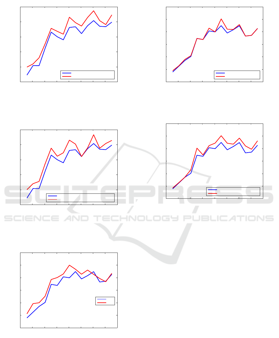
Next, several results for Example 4.4, with various
values of the size parameter N, defining the system or-
der as n = 2N − 1, are presented. The figures below
show the performance for values set as N = 11 : 10 :
151. The problem difficulty increases with increasing
N. For N ∈ { 111, 121,131,151}, care gave a warn-
ing: “Solution may be inaccurate due to poor scaling
or eigenvalues near the stability boundary”. Since the
exact solution is unknown, care results are used as a
reference for obtaining the relative errors. Figure 14
shows the relative errors for Example 4.4, with values
N given above, using scare solver with the best op-
tions. The errors increase from about 10
−13
to 10
−8
,
but the variation is not monotonic. Similarly, the rela-
tive errors for MATLAB R2020b vary from less than
ICINCO 2021 - 18th International Conference on Informatics in Control, Automation and Robotics
86

0 20 40 60 80 100 120 140 160
N
10
-14
10
-12
10
-10
10
-8
10
-6
10
-4
Relative errors
Relative errors to care solution for CAREX 4.4, size N
scare all approaches
scare Hamiltonian pencil approach
Figure 17: Relative errors for Example 4.4 from the
CAREX collection, with various values N, using scare
solver, with Hamiltonian pencil approach and the best op-
tions;
care solution is used as a reference.
0 20 40 60 80 100 120 140 160
N
10
-14
10
-12
10
-10
10
-8
10
-6
10
-4
Relative errors
Relative errors to care solution for CAREX 4.4, size N
scare all approaches
scare skew-Hamiltonian/Hamiltonian approach
Figure 18: Relative errors for Example 4.4 from the
CAREX collection, with various values N, using scare
solver, with skew-Hamiltonian/Hamiltonian approach and
the best options; care solution is used as a reference.
0 20 40 60 80 100 120 140 160
N
10
-14
10
-12
10
-10
10
-8
10
-6
10
-4
10
-2
Relative residuals
Relative residuals for CAREX 4.4, size N
scare
care
Figure 19: Relative residuals for Example 4.4 from the
CAREX collection, with various values N, using MATLAB
function care and scare solver, with the best options.
10
−12
to over 10
−6
.
Figure 15 compares the smallest relative errors
obtained by scare for each value N above, using
0 20 40 60 80 100 120 140 160
N
10
-14
10
-12
10
-10
10
-8
10
-6
10
-4
10
-2
Relative residuals
Relative residuals to care solution for CAREX 4.4, size N
scare all approaches
scare Hamiltonian approach
Figure 20: Relative residuals for Example 4.4 from the
CAREX collection, with various values N, using scare
solver, with Hamiltonian approach and the best options.
0 20 40 60 80 100 120 140 160
N
10
-14
10
-12
10
-10
10
-8
10
-6
10
-4
10
-2
Relative residuals
Relative residuals to care solution for CAREX 4.4, size N
scare all approaches
scare Hamiltonian pencil approach
Figure 21: Relative residuals for Example 4.4 from the
CAREX collection, with various values N, using scare
solver, with Hamiltonian pencil approach and the best op-
tions.
Hamiltonian approach, with the best
scare relative
errors for all approaches, options, and parameters.
For N ∈ {21,31,41,111,121,131,141}, Hamiltonian
approach gives the best results. Figure 16 shows sim-
ilarly the results for MATLAB R2020b.
Figure 17 displays the relative errors using scare
solver with the best options and with Hamiltonian
pencil approach; the latter never wins. Figure 18 plots
the relative errors using scare solver with the best
options and with skew-Hamiltonian/Hamiltonian ap-
proach. The errors coincide for N = 101. Note that
the two pencils approaches do not try the options “no
balancing” and “balancing using an adaptation of the
MATLAB function
arescale ” for this example.
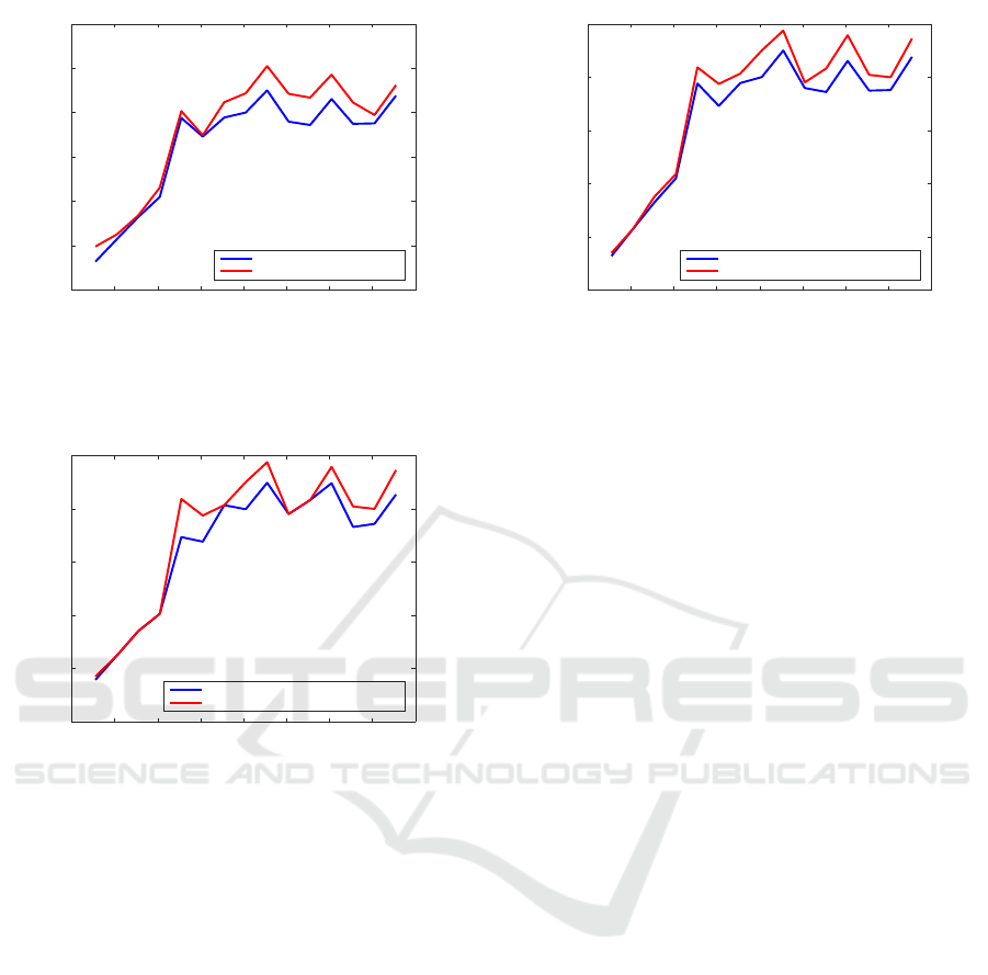
Figure 19 displays the relative residuals using
MATLAB function care and scare solver, with the
best options; scare obtains (slightly) larger residuals
only for N ∈ { 121, 141}, but gains more than one or-
der of magnitude improvements for N ∈ {21, 61,81}.
Figure 20 compares the smallest relative residu-
als obtained by scare using Hamiltonian approach,
A Flexible Structured Solver for Continuous-time Algebraic Riccati Equations
87

0 20 40 60 80 100 120 140 160
N
10
-14
10
-12
10
-10
10
-8
10
-6
10
-4
10
-2
Relative residuals
Relative residuals to care solution for CAREX 4.4, size N (R2020b)
scare all approaches
scare Hamiltonian pencil approach
Figure 22: Relative residuals for Example 4.4 from the
CAREX collection, with various values N, using scare
solver, with Hamiltonian pencil approach and the best op-
tions (MATLAB R2020b).
0 20 40 60 80 100 120 140 160
N
10
-14
10
-12
10
-10
10
-8
10
-6
10
-4
Relative residuals
Relative residuals to care solution for CAREX 4.4, size N
scare all approaches
scare skew-Hamiltonian/Hamiltonian approach
Figure 23: Relative residuals for Example 4.4 from the
CAREX collection, with various values N, using scare
solver, with skew-Hamiltonian/Hamiltonian approach and
the best options.
with the best results of
scare for all approaches,
options, and parameters. The residuals coincide for
N ∈ {51, 61,81, 131,141, 151}.
Figure 21 compares the smallest relative resid-
uals obtained by scare using Hamiltonian pen-
cil approach, with the best results of scare for
all approaches, options, and parameters. For this
test, the Hamiltonian pencil approach has always
larger residuals than
scare solver with the best
choices. However, the differences are of the order
of 10
−13
for small sizes (N ≤ 31). The results for
MATLAB R2020b are similar, see Fig. 22.
Figure 23 compares the smallest rela-
tive residuals obtained by scare using skew-
Hamiltonian/Hamiltonian approach, with the
best results of scare for all approaches, op-
tions, and parameters. The values coincide for
N ∈ {21,31,41, 71,101, 111}, but are larger for the
skew-Hamiltonian/Hamiltonian approach for the
remaining values of N. Figure 24 shows similarly
0 20 40 60 80 100 120 140 160
N
10
-14
10
-12
10
-10
10
-8
10
-6
10
-4
Relative residuals
Relative residuals to care solution for CAREX 4.4, size N (R2020b)
scare all approaches
scare skew-Hamiltonian/Hamiltonian approach
Figure 24: Relative residuals for Example 4.4 from the
CAREX collection, with various values N, using scare
solver, with skew-Hamiltonian/Hamiltonian approach and
the best options (MATLAB R2020b).
the results for MATLAB R2020b. The values
coincide for N = 21, but are larger for the skew-
Hamiltonian/Hamiltonian approach and the other
values of N.
5 CONCLUSIONS
A new, flexible structured solver for continuous-
time algebraic Riccati equations has been pro-
posed and investigated. It can use in an au-
tomatic or specified mode a structured approach
(Hamiltonian matrix, Hamiltonian pencil, or skew-
Hamiltonian/Hamiltonian pencil), an orthogonaliza-
tion method (QR, QR with pivoting, or SVD), a bal-
ancing option and its threshold parameter. The solver
can be used in a loop over the approaches, methods,
options and parameters to obtain the solution with
minimum relative error (with respect to a known or
reference solution) and a possibly different solution
with minimum relative residual. It has been applied
for solving the examples from the SLICOT CAREX
benchmark collection. The numerical results illus-
trate its very good performance in comparison with
the state-of-the-art MATLAB solver.
REFERENCES
Abels, J. and Benner, P. (1999). CAREX—A collection
of benchmark examples for continuous-time algebraic
Riccati equations (Version 2.0). SLICOT Working
Note 1999-14. Available from www.slicot.org .
Anderson, E., Bai, Z., Bischof, C., Blackford, S., Demmel,
J., Dongarra, J., Du Croz, J., Greenbaum, A., Ham-
marling, S., McKenney, A., and Sorensen, D. (1999).
LAPACK Users’ Guide: Third Edition. Software · En-
vironments · Tools. SIAM, Philadelphia.
ICINCO 2021 - 18th International Conference on Informatics in Control, Automation and Robotics
88

Bender, D. J. and Laub, A. J. (1987a). The linear-quadratic
optimal regulator for descriptor systems. IEEE Trans.
Automat. Contr., AC-32(8):672–688.
Bender, D. J. and Laub, A. J. (1987b). The linear-quadratic
optimal regulator for descriptor systems: Discrete-
time case. Automatica, 23(1):71–85.
Benner, P. (2001). Symplectic balancing of Hamiltonian
matrices. SIAM J. Sci. Comput., 22(5):1885–1904.
Benner, P., Byers, R., Losse, P., Mehrmann, V., and
Xu, H. (2007). Numerical solution of real skew-
Hamiltonian/Hamiltonian eigenproblems. Technical
report, Technische Universit
¨
at Chemnitz, Chemnitz.
Benner, P., Byers, R., Mehrmann, V., and Xu, H. (2002).
Numerical computation of deflating subspaces of
skew Hamiltonian/Hamiltonian pencils. SIAM J. Ma-
trix Anal. Appl., 24(1):165–190.
Benner, P., Kressner, D., Sima, V., and Varga, A. (2010).
Die SLICOT-Toolboxen f
¨
ur Matlab. at — Automa-
tisierungstechnik, 58(1):15–25.
Benner, P., Mehrmann, V., Sima, V., Van Huffel, S., and
Varga, A. (1999). SLICOT — A subroutine library in
systems and control theory. In Datta, B. N. (ed.), Ap-
plied and Computational Control, Signals, and Cir-
cuits, vol. 1, 499–539. Birkh
¨
auser, Boston, MA.
Benner, P., Mehrmann, V., and Xu, H. (1997). A new
method for computing the stable invariant subspace
of a real Hamiltonian matrix. J. Comput. Appl. Math.,
86(1):17–43.
Benner, P., Mehrmann, V., and Xu, H. (1998). A numeri-
cally stable, structure preserving method for comput-
ing the eigenvalues of real Hamiltonian or symplectic
pencils. Numer. Math., 78(3):329–358.
Benner, P. and Sima, V. (2003). Solving algebraic Riccati
equations with SLICOT. In MED’03, 11th Mediter-
ranean Conference on Control and Automation.
Benner, P., Sima, V., and Voigt, M. (2016). Al-
gorithm 961: Fortran 77 subroutines for the so-
lution of skew-Hamiltonian/Hamiltonian eigenprob-
lems. ACM Transactions on Mathematical Software
(TOMS), 42(3):1–26.
Bojanczyk, A. W., Golub, G., and Van Dooren, P. (1992).
The periodic Schur decomposition: Algorithms and
applications. In SPIE Conference Advanced Signal
Processing Algorithms, Architectures, and Implemen-
tations III, vol. 1770, 31–42.
Granat, R., K
˚
agstr
¨
om, B., and Kressner, D. (2007a). Com-
puting periodic deflating subspaces associated with a
specified set of eigenvalues. BIT Numerical Mathe-
matics, 47(4):763–791.
Granat, R., K
˚
agstr
¨
om, B., and Kressner, D. (2007b). MAT-
LAB tools for solving periodic eigenvalue problems.
In Third IFAC Workshop on Periodic Control Systems.
Lancaster, P. and Rodman, L. (1995). The Algebraic Riccati
Equation. Oxford University Press, Oxford.
MathWorks
®
(2015). Control System Toolbox
™
, Release
R2015b.
MathWorks
®
(2016). MATLAB
®
Primer. R2016a. The
MathWorks, Inc., Natick, MA.
Mehrmann, V. (1991). The Autonomous Linear Quadratic
Control Problem. Theory and Numerical Solution.
Springer-Verlag, Berlin.
Sima, V. (1996). Algorithms for Linear-Quadratic Opti-
mization. Marcel Dekker, Inc., New York.
Sima, V. (2010). Structure-preserving computation of sta-
ble deflating subspaces. In ALCOSP 2010, 10th IFAC
Workshop “Adaptation and Learning in Control and
Signal Processing”.
Sima, V. (2011). Computational experience with structure-
preserving Hamiltonian solvers in optimal control. In
ICINCO 2011, 8th International Conference on Infor-
matics in Control, Automation and Robotics, vol. 1,
91–96. SciTePress.
Sima, V. (2016). Balancing skew-Hamiltonian/Hamiltonian
pencils with applications in control engineering. In
ICINCO-2016, 13th International Conference on In-
formatics in Control, Automation and Robotics, vol. 1,
177–184. SciTePress.
Sima, V. (2019). Computation of initial transformation for
implicit double step in the periodic QZ algorithm. In
ICSTCC 2019, 23th International Conference on Sys-
tem Theory, Control and Computing, 7–12. IEEE.
Sima, V. and Benner, P. (2015a). Pitfalls when solving
eigenproblems with applications in control engineer-
ing. In ICINCO-2015, 12th International Conference
on Informatics in Control, Automation and Robotics,
vol. 1, 171–178. SciTePress.
Sima, V. and Benner, P. (2015b). Solving SLICOT bench-
marks for continuous-time algebraic Riccati equations
by Hamiltonian solvers. In ICSTCC 2015, 19th Inter-
national Conference on System Theory, Control and
Computing, 1–6. IEEE.
Sima, V. and Benner, P. (2016). Improved balancing for
general and structured eigenvalue problems. In IC-
STCC 2016, 20th International Conference on System
Theory, Control and Computing, 381–386. IEEE.
Sima, V. and Gahinet, P. (2019). Improving the conver-
gence of the periodic QZ algorithm. In ICINCO-
2019, 16th International Conference on Informatics
in Control, Automation and Robotics, vol. 1, 261–268.
SciTePress.
Sima, V. and Gahinet, P. (2020). Using semi-implicit itera-
tions in the periodic QZ algorithm. In ICINCO-2020,
17th International Conference on Informatics in Con-
trol, Automation and Robotics, vol. 1: ICINCO, 35–
46. SciTePress.
Sreedhar, J. and Van Dooren, P. (1994). Periodic Schur
form and some matrix equations. In MTNS’93, Sys-
tems and Networks: Mathematical Theory and Appli-
cations, vol. 1, 339–362. John Wiley & Sons.
Van Dooren, P. (1981). A generalized eigenvalue approach
for solving Riccati equations. SIAM J. Sci. Stat. Com-
put., 2(2):121–135.
Xu, H. (2006). On equivalence of pencils from discrete-
time and continuous-time control. Lin. Alg. Appl.,
414(1):97–124.
A Flexible Structured Solver for Continuous-time Algebraic Riccati Equations
89