Comparison of Different Radial Basis Functions in Dynamical Systems
∗
Arg
´
aez
1 a
, Peter Giesl
2 b
and Sigurdur Hafstein
1 c
1
Science Institute, University of Iceland, Dunhagi 3, 107 Reykjav
´
ık, Iceland
2
Department of Mathematics, University of Sussex, Falmer, BN1 9QH, U.K.
Keywords:
Generalised Interpolation, Radial Basis Functions, Complete Lyapunov Functions.
Abstract:
In this paper we study the impact of using different radial basis functions for the computation of complete
Lyapunov function candidates using generalised interpolation. We compare the numerical well-posedness
of the discretised problem, condition numbers of the collocation matrices, and the quality of the solutions
for Wendland functions ψ
3,1
and ψ
5,3
, Gaussians, Inverse quadratics and Inverse multiquadrics, and Mat
´
ern
kernels ψ
(n+3)/2
and ψ
(n+5)/2
.
1 INTRODUCTION
Radial basis functions (RBFs) are a standard tool for
interpolation and generalised interpolation problems
in high dimensions. One of the applications in the
area of Dynamical Systems is the computation of Lya-
punov functions (Giesl, 2007a; Giesl and Wendland,
2007), as well as complete Lyapunov function can-
didates (Arg
´
aez et al., 2017a; Arg
´
aez et al., 2017b;
Arg
´
aez et al., 2018a; Arg
´
aez et al., 2018b). This
is formulated as a generalised interpolation problem,
approximately solving a suitable linear, first-order
partial differential equation (PDE).
Let us explain the computation of complete Lya-
punov function candidates for dynamical systems in
more detail, where the dynamics are given by the au-
tonomous ordinary differential equation (ODE)
˙
x =
f(x) with x ∈ R
n
. Our initial method computes
a complete Lyapunov function candidate V as the
generalised interpolant to the linear, first-order PDE
∇V (x)·f(x) = −1. Note, however, that the PDE is ill-
posed, as it does not have a solution at certain points
x, namely in the chain-recurrent set, i.e. where the dy-
namics are repetitive or almost repetitive, which in-
cludes equilibria and periodic orbits. However, this
apparent disadvantage of the method is used to obtain
information on the location of the chain-recurrent set
a
https://orcid.org/0000-0002-0455-8015
b
https://orcid.org/0000-0003-1421-6980
c
https://orcid.org/0000-0003-0073-2765
∗
This paper is supported by the Icelandic Research Fund
(Rann
´
ıs) grant number 1163074-052, Complete Lyapunov
functions: Efficient numerical computation.
of the ODE. This information can then be used for
further iterations to obtain complete Lyapunov func-
tion candidates localising the chain-recurrent set with
more precision.
The RBFs that have mainly been used for the
computation of complete Lyapunov function candi-
dates are Wendland’s RBFs. They are positive definite
and polynomials on their compact support and their
smoothness is fixed through a parameter. The corre-
sponding reproducing kernel Hilbert space (RKHS),
where the mesh-free collocation is performed and the
norm of which is minimised, is norm-equivalent to a
Sobolev space. Usually Wendland functions with low
smoothness parameters are used and the method in
(Arg
´
aez et al., 2017a; Arg
´
aez et al., 2017b; Arg
´
aez
et al., 2018a; Arg
´
aez et al., 2018b) to compute com-
plete Lyapunov functions candidates works very well.
However, any sufficiently smooth RBF can be used.
Indeed, in theory the smoother the RBFs, the bet-
ter the convergence results, but in applications less
smooth RBFs often work better, since they avoid nu-
merical problems as shown in this paper.
A natural question is thus how the method works
in practice with different RBFs. In this paper we sys-
tematically analyse several candidates for RBFs and
compare three aspects relevant to the applicability.
All the RBFs we analyse depend on a positive real
parameter c and the influence of the value of the pa-
rameter must also be taken into account. Further, the
density of the collocation points in the generalised
interpolation problem plays a vital role. To make
the analysis tractable we compute complete Lyapunov
function candidates for a system with a known chain-
394
Argáez, C., Giesl, P. and Hafstein, S.
Comparison of Different Radial Basis Functions in Dynamical Systems.
DOI: 10.5220/0010575203940405
In Proceedings of the 11th International Conference on Simulation and Modeling Methodologies, Technologies and Applications (SIMULTECH 2021), pages 394-405
ISBN: 978-989-758-528-9
Copyright
c
 2021 by SCITEPRESS – Science and Technology Publications, Lda. All rights reserved

recurrent set; two periodic orbits and one equilibrium.
The three aspects we analyse are:
First, the collocation matrix generated for the dis-
cretised problem is symmetric and should in theory
be positive definite. If it is not positive definite due
to numerical issues, then it is not possible to compute
a solution to the discretised problem and the method
cannot work. We analyse the positive definiteness of
the collocation matrix as a function of the RBF pa-
rameter c > 0 and the density of the collocation grid
parameterised through α > 0, cf. formula (9) below.
Second, the condition number of the collocation
matrix is of great relevance to the method, in partic-
ular when iterating. Thus, we also analyse the condi-
tion number of the collocation matrix as a function of
the RBF parameter c > 0 and the density of the collo-
cation grid α.
Third, since we know the location of the chain-
recurrent set, we analyse how well it is localised by
the method using the different RBFs. Again the RBF
parameter c > 0 and the density of the collocation grid
α play a role. In general, one aims for a good locali-
sation of the chain-recurrent set with as coarse a col-
location grid as possible.
The RBFs we analyse, always with a scaling pa-
rameter c > 0, are the following, for references see,
e.g., (Fasshauer, 2007; Wendland, 2005; Schaback,
1993; Buhmann, 2003).
Wendland ψ
3,1
ψ(r) = (1 − cr)
4
+
[4cr + 1] (1)
Recall that x
+
:= max{0,x} and x
k
+
:= (x
+
)
k
. We con-
sider R
2
, so n = 2, and the parameters for the Wend-
land function ψ
l,k
are chosen such that l =

n
2

+
k + 1 = k + 2; the corresponding RKHS is norm-
equivalent to the Sobolev space H
k+(n+1)/2
= H
5/2
.
Wendland ψ
5,3
ψ(r) = (1 − cr)
8
+
[32(cr)
3
+ 25(cr)
2
+ 8cr + 1] (2)
The corresponding RKHS is norm-equivalent to the
Sobolev space H
k+(n+1)/2
= H
9/2
.
Gaussians
ψ(r) = exp

−r
2
2c
2

(3)
Inverse multiquadric
ψ(r) =
1
p
1 + (cr)
2
(4)
Inverse quadratic
ψ(r) =
1
1 + (cr)
2
(5)
Mat
´
ern ψ
(n+3)/2
ψ(r) = (1 + cr)exp(−cr) (6)
Mat
´
ern kernels are well known in the statistics liter-
ature (Matern, 1986) and called Sobolev splines in
(Schaback, 1993). We consider R
2
, so n = 2, and the
parameter for the Mat
´
ern kernel ψ
β
is chosen such
that β =
n+3
2
=
5
2
; the corresponding RKHS is norm-
equivalent to the Sobolev space H
β
= H
5
2
.
Mat
´
ern ψ
(n+5)/2
ψ(r) =

1 + cr +
1
3
(cr)
2

exp(−cr) (7)
We consider R
2
, so n = 2, and the parameter for the
Mat
´
ern kernel ψ
β
is chosen such that β =
n+5
2
=
7
2
;
the corresponding RKHS is norm-equivalent to the
Sobolev space H
β
= H
7
2
.
Remark 1.1. Note that although all the RBFs studied
are parameterised by a parameter c > 0, this param-
eter has different meanings for different RBFs and its
numerical values cannot be directly compared.
The paper is organised as follows: In the next
section we give a brief description of the method
to compute complete Lyapunov function candidates
from (Giesl, 2007b) refined in (Arg
´
aez et al., 2017a;
Arg
´
aez et al., 2017b; Arg
´
aez et al., 2018a; Arg
´
aez
et al., 2018b), before we present our results in Sec-
tion 3 and discuss them in Section 4.
In this paper we are only interested in the per-
formance of different RBFs to obtain complete Lya-
punov functions. Therefore, one iteration suffices.
2 USING RBFs TO COMPUTE
COMPLETE LYAPUNOV
FUNCTION CANDIDATES
The method used to compute complete Lyapunov
function candidates using generalised interpolation
with RBFs is described in detail in (Arg
´
aez et al.,
2017a; Arg
´
aez et al., 2017b; Arg
´
aez et al., 2018a;
Arg
´
aez et al., 2018b). Here we just give a brief
overview. Given is a dynamical system, whose dy-
namics are defined by an ODE
˙
x = f(x), f : R
n
→ R
n
, (8)
and we are interested in the qualitative behaviour of
its solution t 7→ φ(t,ξ) as a function of the initial value
ξ ∈ R
n
; here φ(0,ξ) = ξ and
˙
φ(t,ξ) = f(φ(t, ξ)). The
qualitative behaviour of the solutions is characterised
by a so-called complete Lyapunov function for the
system V : R
n
→ R, which is non-increasing along
all solution trajectories, and strictly decreasing where
possible, cf. (Auslander, 1964; Conley, 1978; Hurley,
1998). A complete Lyapunov function candidate is
Comparison of Different Radial Basis Functions in Dynamical Systems
395

a function, which fulfills the first property, namely
that it is non-increasing along all solution trajecto-
ries. This can be expressed by a non-positive orbital
derivative (derivative along solutions) ∇V(x) · f(x) ≤
0, if V is sufficiently smooth.
It was shown in (Arg
´
aez et al., 2018a) that it
is advantageous to homogenise the solutions’ speed
while maintaining the same trajectories by substitut-
ing
ˆ
f(x) = f(x)/
p
δ
2
+ kf(x)k
2
for f in (8), where
δ > 0 is a small parameter. We set δ
2
= 10
−8
in our
computations.
The computation of complete Lyapunov function
candidates is then posed as a generalised interpola-
tion problem and solved using a collocation method
based on RBFs. The set of collocation points X =
{x
1
,...,x
N
} ⊂ R
n
is a subset of a, possibly shifted,
hexagonal grid
(
α
n
∑
k=1
i
k
ω
k
: i
k
∈ Z
)
, where (9)
ω
k
=
k−1
∑
j=1
ε
j
e
j
+ (k + 1)ε
k
e
k
and ε
k
=
s
1
2k(k +1)
.
In the formula e
j
is the usual jth unit vector and the
parameter α > 0 is a measure of the density; small
α > 0 correspond to high density. Further, we re-
quire f(x
i
) 6= 0 for any x
i
∈ X to obtain a positive defi-
nite collocation matrix. This hexagonal grid has been
shown to minimise the condition numbers of the col-
location matrices for a fixed fill distance (Iske, 1998).
Next we compute the generalised interpolant v
to v
0
(x
i
) := ∇v(x
i
) · f(x
i
) = −p(x
i
) at all collocation
points x
i
∈ X; v
0
(x
i
) := ∇v(x
i
) · f(x
i
) is the so-called
orbital derivative of the function v and is negative if
v is decreasing along solution trajectories of the ODE
(8). The generalised interpolant is known to be the
norm-minimal function in the corresponding RKHS
fulfilling the interpolation conditions v
0
(x
i
) = −p(x
i
).
It is computed by solving a system of linear equations
with a collocation matrix.
For details we refer to (Arg
´
aez et al., 2017a;
Arg
´
aez et al., 2018a; Arg
´
aez et al., 2018b) or (Giesl,
2007b, Chapter 3). In the first iteration we start with
the right-hand side p(x
i
) = 1 for all x
i
∈ X. Once we
have computed the generalised interpolant v we eval-
uate v
0
(x) on a grid Y
x
i
along the flow at each colloca-
tion point x
i
∈ X and use this information to fix p(x
i
)
in the next iteration, cf. (Arg
´
aez et al., 2018b).
A complete Lyapunov function V : R
n
→ R for the
ODE (8) fulfills V
0
(x) ≤ 0 for all x ∈ R
n
and V
0
(x) < 0
whenever possible. The set of x ∈ R
n
where V
0
(x) = 0
corresponds to (almost) recurrent motion and is called
the chain-recurrent set. At points that are not in the
chain-recurrent set the flow of the ODE is gradient-
like, i.e. solutions flow through and do not return to
a neighbourhood of the point. The method outlined
above computes a complete Lyapunov function candi-
date v and can be used to localise the chain-recurrent
set. There are different methods to do that; here we
use the criterion that k∇v(x)k ≤ γ
+
for some (small)
parameter γ
+
(Arg
´
aez et al., 2021).
3 RESULTS
For all the tests we used the ODE
f(x,y) =

−x(x
2
+ y
2
− 1/4)(x
2
+ y
2
− 1) − y
−y(x
2
+ y
2
− 1/4)(x
2
+ y
2
− 1) + x

,
(10)
which has an asymptotically stable equilibrium at the
origin and two circular periodic orbits centred at the
origin; a repelling one with radius 1/2 and an asymp-
totically stable one with radius 1. The chain-recurrent
set of the system consists of these three components.
With the method outlined in the last section one ex-
pects to obtain an estimate of the chain-recurrent set
that covers the three components, i.e. the origin and
the two circles centred at the origin with radius 1/2
and 1, and preferably the estimate is reasonably tight.
In the following the collocation points are always
the hexagonal grid from formula (9), shifted as in
(Hafstein, 2017) and intersected with [−1.5,1.5]
2
. To
localise the chain-recurrent set we evaluated v
0
on the
dense regular grid (∆x Z × ∆y Z) ∩ [−1.5,1.5]
2
with
∆x = ∆y = 0.02. In all examples we analyse the chain-
recurrent set of the complete Lyapunov function for
different values of c and α. The different columns in
the figures show combinations of α and c resulting
in condition numbers 10
3
, 10
6
and 10
13
, respectively.
Note that the condition number increases, while the
error decreases, if we either decrease α (denser set of
collocation points) or if we decrease c (larger over-
lap). The chain-recurrent set was approximated as the
set of points x fulfilling k∇v
0
(x)k ≤ γ
+
= 0.2 for all
examples. Table 1 shows the parameters used for our
computations.
3.1 Wendland ψ
3,1
We consider the Wendland function ψ
3,1
from (1)
with scaling parameter c > 0. The collocation ma-
trix is always positive definite for all choices of c > 0
(scaling parameter) and α (density of the hexagonal
collocation grid) that we investigated, namely 0.1 ≤
c ≤ 10 and 0.02 ≤ α ≤ 1. Figures 1 and 2 show
the computed chain-recurrent set for system (10). All
computations show very good approximations of the
SIMULTECH 2021 - 11th International Conference on Simulation and Modeling Methodologies, Technologies and Applications
396

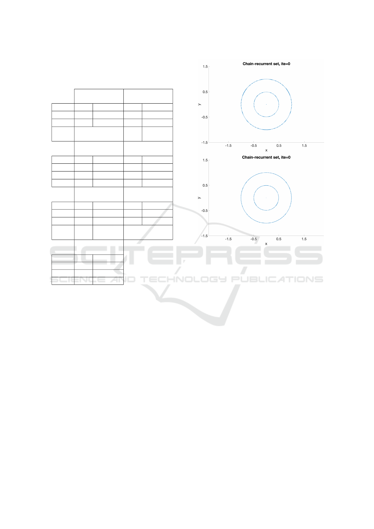
Table 1: Different parameters for α and c used according
to the radial basis functions. Parameters were chosen to
reproduce similar condition numbers (cond.) in the corre-
sponding collocation matrices.
Wendland func.
ψ
3,1
Wendland func.
ψ
5,3
Cond.
α c α c
10
3
0.06 1 0.03 7
10
5
0.03 1 0.03 2.5
10
13
Not reached
with our settings
0.03 0.2
Gaussian
function
Inverse
Multiquadrics
Cond.
α c α c
10
3
0.12 0.1 0.14 4
10
5
0.39 0.6 0.51 0.4
10
13
0.05 0.1 0.55 0.1
Inverse
Quadratic
Mat
´
ern
ψ
(n+3)/2
Cond.
α c α c
10
3
0.2 2.4 0.3 0.3
10
5
0.41 0.5 0.03 0.3
10
13
0.08 1.5
Not reached
with our settings
Mat
´
ern
ψ
(n+5)/2
Cond.
α c
10
3
0.16 5.3
10
5
0.07 2.9
10
13
0.03 0.1
chain-recurrent set, which consists of two circles of
radii 1/2 and 1 and a point at the origin. Iteration 1 is
better than iteration 0. The upper figure with higher
condition number produces a slightly clearer approx-
imation of the chain-recurrent set than the lower fig-
ure.
3.2 Wendland ψ
5,3
We consider the Wendland function ψ
5,3
from (2)
with scaling parameter c > 0. Again the collocation
matrix is positive definite for all choices of c > 0
(scaling parameter) and α (density of the hexagonal
collocation grid) that we investigated, namely 0.1 ≤
c ≤ 10 and 0.02 ≤ α ≤ 1. Figures 3 (iteration 0) and
4 (iteration 1) show the approximation of the chain-
recurrent set for system (10) using ψ
5,3
. The lowest
condition number (top) shows an over-estimation of
the chain-recurrent set in iteration 1, the medium con-
dition (middle) shows an under-estimation. The best
result is given by the largest condition number in iter-
ation 1, Figure 4 bottom.
Figure 1: Chain-recurrent set from the approximation with
Wendland function 3,1 in iteration 0 with collocation matrix
with condition number 10
3
(upper) and 10
5
(lower).
3.3 Gaussian Radial Basis Functions
We consider the Gaussian RBF functions (3) with
scaling parameter c > 0. Figure 15 shows that the
collocation matrix is positive definite only for certain
choices of c > 0 (scaling parameter) and α (density
of the hexagonal collocation grid). Figures 5 and 6
show that the approximation of the chain-recurrent set
is poor in all cases.
3.4 Inverse Multiquadrics
We consider the Inverse multiquadrics (4) with scal-
ing parameter c > 0. In Figure 16 it can be seen the
collocation matrix is positive definite only for certain
choices of c > 0 (scaling parameter) and α (density
of the hexagonal collocation grid). Figures 7 and 8
suggest that the best results are obtained with matri-
ces whose condition number is small and even then
the results are inferior to those of the Wendland func-
tions.
Comparison of Different Radial Basis Functions in Dynamical Systems
397

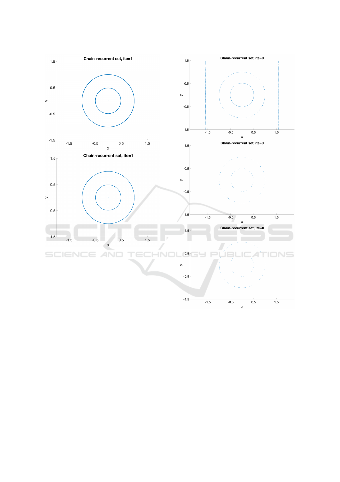
Figure 2: Chain-recurrent set from the approximation with
Wendland function 3,1 in iteration 1 with collocation matrix
with condition number 10
3
(upper) and 10
5
(lower).
3.5 Inverse Quadratic
We consider the Inverse quadratics (5) with scaling
parameter c > 0. In Figure 17 we see that the colloca-
tion matrix is positive definite only for certain choices
of c and α. Figures 9 and 10 show, similar to the
Inverse multiquadrics, that better results are obtained
for matrices with small condition number. But even
then the approximation of the chain-recurrent set is
poor and inferior to the case of Wendland functions.
3.6 Mat
´
ern ψ
(n+3)/2
We consider the Mat
´
ern kernel ψ
(n+3)/2
from (6) with
scaling parameter c > 0. The collocation matrix is
positive definite for all choices of c and α that we in-
vestigated, namely 0.1 ≤ c ≤ 10 and 0.02 ≤ α ≤ 1.
Figures 11 and 12 show good estimates for the larger
condition number, while the smaller condition num-
ber delivers an over-estimation in iteration 0 and a
completely wrong result in iteration 1.
Figure 3: Chain-recurrent set from the approximation with
Wendland function 5,3 in iteration 0 with collocation matrix
with condition numbers 10
3
(top), 10
5
(middle), and 10
13
(bottom).
3.7 Mat
´
ern ψ
(n+5)/2
We consider the Mat
´
ern kernel ψ
(n+5)/2
from (7). The
collocation matrix is positive definite for all choices
of c and α that we investigated, namely 0.1 ≤ c ≤ 10
and 0.02 ≤ α ≤ 1. Figures 13 and 14 show better
approximations of the chain-recurrent set than with
Mat
´
ern ψ
(n+3)/2
, in particular in iteration 0. The
lower the condition number, the better the results,
with some gaps in the circles for large condition num-
bers.
SIMULTECH 2021 - 11th International Conference on Simulation and Modeling Methodologies, Technologies and Applications
398

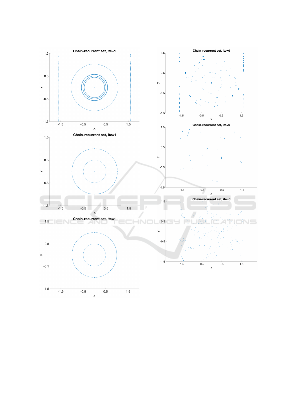
Figure 4: Chain-recurrent set from the approximation with
Wendland function 5,3 in iteration 1 with collocation matrix
with condition numbers 10
3
(top), 10
5
(middle), and 10
13
(bottom).
3.8 Comparison of All the Functions
In Figure 18 all the radial basis functions used are
plotted for the parameter c = 1. The Wendland func-
tions have a compact support and fall more rapidly
than the other functions.
Figure 5: Chain-recurrent set from the approximation with
the Gaussians in iteration 0 with collocation matrix with
condition numbers 10
3
(top), 10
5
(middle), and 10
13
(bot-
tom).
4 DISCUSSION
The results from our numerical investigation can be
summarized as follows: The Wendland and Mat
´
ern
functions share a similar behaviour concerning the
area in the α vs. c plane for positive definite matri-
ces: most of the combinations of different α and c pa-
rameters numerically produce positive definite matri-
ces. The other radial basis functions (RBFs), namely
Gaussians, Inverse multiquadrics and Inverse quadrat-
Comparison of Different Radial Basis Functions in Dynamical Systems
399

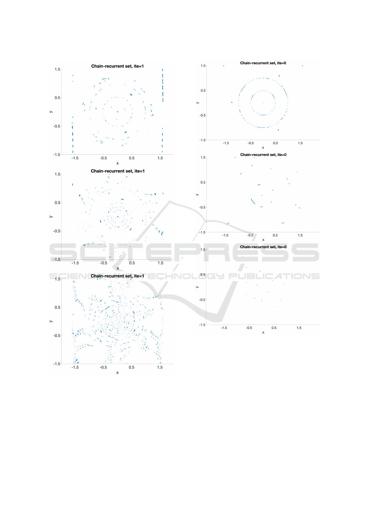
Figure 6: Chain-recurrent set from the approximation with
the Gaussians in iteration 1 with collocation matrix with
condition numbers 10
3
(top), 10
5
(middle), and 10
13
(bot-
tom).
ics, have a limited region of parameter values lead-
ing to (numerically) positive definite collocation ma-
trices.
Summarizing, the best results, both in terms of
positive definite matrices and the accuracy of the
Figure 7: Chain-recurrent set from the approximation with
the Inverse multiquadrics in iteration 0 with collocation ma-
trix with condition numbers 10
3
(top), 10
5
(middle), and
10
13
(bottom).
chain-recurrent sets, were obtained for Wendland
functions and Mat
´
ern kernels. These are kernels with
a low degree of smoothness. For the smoother ker-
nels, the matrices become numerically problematic
quickly, i.e. not positive definite, when using denser
collocation grids, while at the same time the localisa-
tion of the chain-recurrent set is poor.
This is a somewhat surprising result, since theoret-
ical error estimates suggest that using smoother RBFs
results in faster convergence; however, numerically,
the collocation matrices quickly become non-positive
SIMULTECH 2021 - 11th International Conference on Simulation and Modeling Methodologies, Technologies and Applications
400

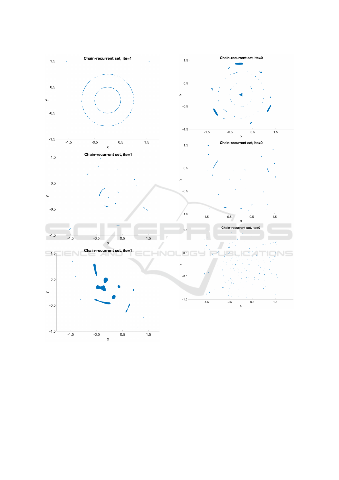
Figure 8: Chain-recurrent set from the approximation with
the Inverse multiquadrics in iteration 1 with collocation ma-
trix with condition numbers 10
3
(top), 10
5
(middle), and
10
13
(bottom).
definite. Our study confirms that Wendland func-
tions are a good choice as RBFs for our application in
Dynamical Systems to compute complete Lyapunov
function candidates, and are preferable to Gaussians,
Inverse quadratics and Inverse multiquadrics. More-
Figure 9: Chain-recurrent set from the approximation with
the Inverse quadratics in iteration 0 with collocation matrix
with condition numbers 10
3
(top), 10
5
(middle), and 10
13
(bottom).
over, the Mat
´
ern kernels are also promising RBFs for
our application and their use should be explored fur-
ther.
Comparison of Different Radial Basis Functions in Dynamical Systems
401

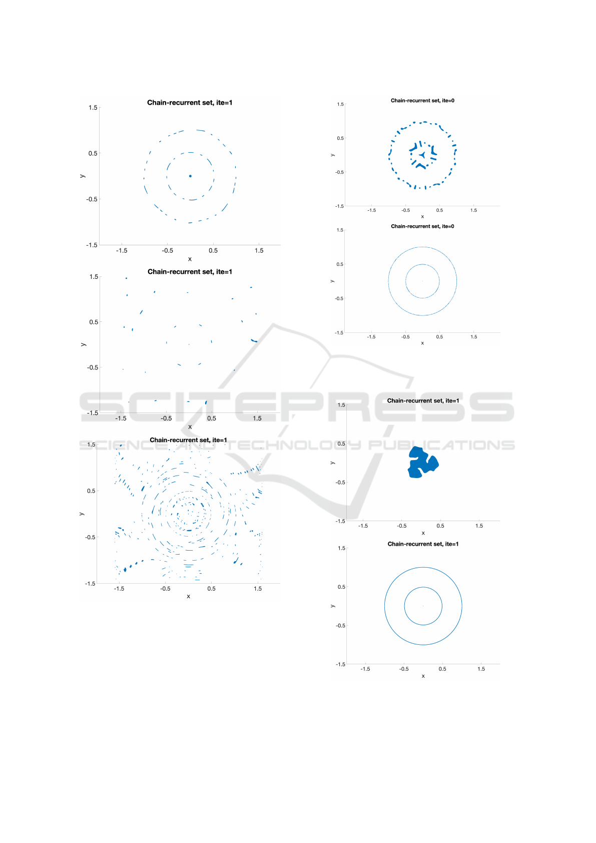
Figure 10: Chain-recurrent set from the approximation with
the Inverse quadratics in iteration 1 with collocation matrix
with condition numbers 10
3
(top), 10
5
(middle), and 10
13
(bottom).
Figure 11: Chain-recurrent set from the approximation with
Mat
´
ern ψ
(n+3)/2
kernels in iteration 0 with collocation ma-
trix with condition number 10
3
(upper) and 10
5
(lower).
Figure 12: Chain-recurrent set from the approximation with
Mat
´
ern ψ
(n+3)/2
kernels in iteration 1 with collocation ma-
trix with condition number 10
3
(upper) and 10
5
(lower).
SIMULTECH 2021 - 11th International Conference on Simulation and Modeling Methodologies, Technologies and Applications
402

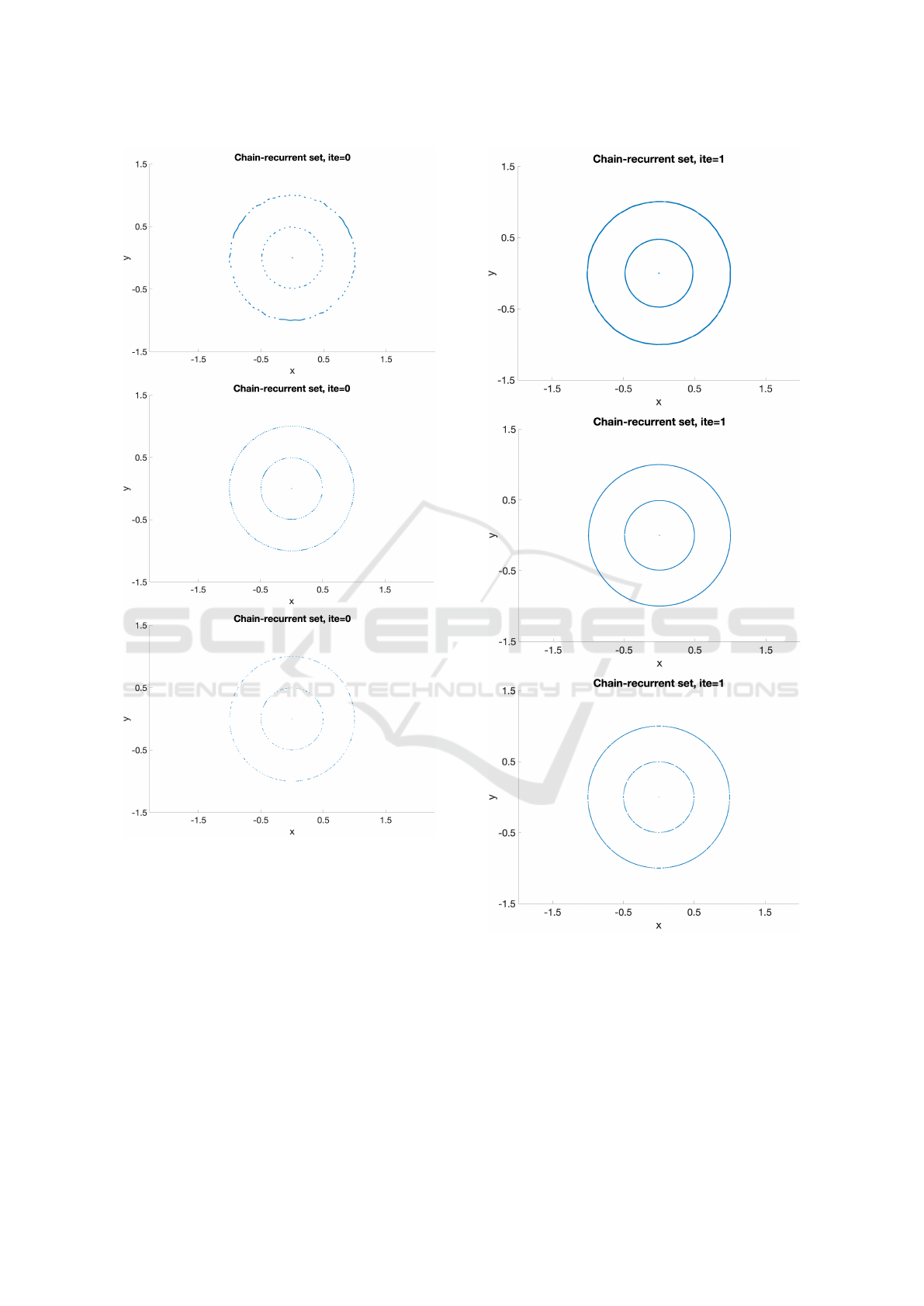
Figure 13: Chain-recurrent set from the approximation with
Mat
´
ern ψ
(n+5)/2
kernels in iteration 0 with collocation ma-
trix with condition numbers 10
3
(top), 10
5
(middle), and
10
13
(bottom).
Figure 14: Chain-recurrent set from the approximation with
Mat
´
ern ψ
(n+5)/2
kernels in iteration 1 with collocation ma-
trix with condition numbers 10
3
(top), 10
5
(middle), and
10
13
(bottom).
Comparison of Different Radial Basis Functions in Dynamical Systems
403

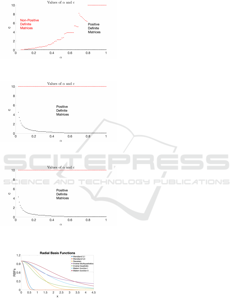
Figure 15: Gaussian RBF: c vs α, for a given α the colloca-
tion matrix is positive definite on the c interval between the
black and the red dot.
Figure 16: Inverse multiquadrics: c vs α, for a given α the
collocation matrix is positive definite on the c interval be-
tween the black and the red dot.
Figure 17: Inverse quadratic RBF: c vs α, for a given α
the collocation matrix is positive definite on the c interval
between the black and the red dot.
Figure 18: Comparison of all the radial basis functions used
with parameter c = 1.
REFERENCES
Arg
´
aez, C., Giesl, P., and Hafstein, S. (2017a). Analysing
dynamical systems towards computing complete Lya-
punov functions. In Proceedings of the 7th In-
ternational Conference on Simulation and Model-
ing Methodologies, Technologies and Applications,
Madrid, Spain, pages 323–330.
Arg
´
aez, C., Giesl, P., and Hafstein, S. (2018a). Dynamical
Systems in Theoretical Perspective, volume 248, chap-
ter Computational approach for complete Lyapunov
functions, pages 1–11. Springer. Springer Proceed-
ings in Mathematics and Statistics.
Arg
´
aez, C., Giesl, P., and Hafstein, S. (2018b). Iterative
construction of complete Lyapunov functions. In Pro-
ceedings of the 8th International Conference on Sim-
ulation and Modeling Methodologies, Technologies
and Applications, pages 211–222.
Arg
´
aez, C., Giesl, P., and Hafstein, S. (2021). Complete
Lyapunov Functions: Determination of the Chain-
recurrent set using the Gradient. In Simulation and
Modeling Methodologies, Technologies and Applica-
tions Series: Advances in Intelligent Systems and
Computing 1260 eds. M. Obaidat, T.
¨
Oren, and F. De
Rango,Springer, pages 104–112.
Arg
´
aez, C., Hafstein, S., and Giesl, P. (2017b). Wendland
functions - a C++ code to compute them. In Proceed-
ings of the 7th International Conference on Simula-
tion and Modeling Methodologies, Technologies and
Applications, pages 323–330.
Auslander, J. (1964). Generalized recurrence in dynamical
systems. Contr. to Diff. Equ., 3:65–74.
Buhmann, M. D. (2003). Radial basis functions: theory
and implementations, volume 12 of Cambridge Mono-
graphs on Applied and Computational Mathematics.
Cambridge University Press, Cambridge.
Conley, C. (1978). Isolated Invariant Sets and the Morse
Index. CBMS Regional Conference Series no. 38.
American Mathematical Society.
Fasshauer, G. (2007). Meshfree approximation methods
with MATLAB. Number 6 in Interdisciplinary Mathe-
matical Sciences. World Scientific Publishing.
Giesl, P. (2007a). Construction of Global Lyapunov Func-
tions Using Radial Basis Functions. Lecture Notes in
Math. 1904, Springer.
Giesl, P. (2007b). Construction of Global Lyapunov Func-
tions Using Radial Basis Functions, volume 1904
of Lecture Notes in Mathematics. Springer-Verlag,
Berlin.
Giesl, P. and Wendland, H. (2007). Meshless collocation:
error estimates with application to Dynamical Sys-
tems. SIAM J. Numer. Anal., 45(4):1723–1741.
Hafstein, S. (2017). Efficient algorithms for simplicial com-
plexes used in the computation of Lyapunov func-
tions for nonlinear systems. In Proceedings of the
7th International Conference on Simulation and Mod-
eling Methodologies, Technologies and Applications
(SIMULTECH), pages 398–409.
Hurley, M. (1998). Lyapunov functions and attractors
SIMULTECH 2021 - 11th International Conference on Simulation and Modeling Methodologies, Technologies and Applications
404

in arbitrary metric spaces. Proc. Amer. Math. Soc.,
126:245–256.
Iske, A. (1998). Perfect centre placement for radial ba-
sis function methods. Technical Report TUM-M9809,
TU Munich, Germany.
Matern, B. (1986). Spatial variation. Lecture Notes in
Statistics. Springer.
Schaback, R. (1993). Comparison of radial basis func-
tion interpolants. Multivariate Approximation: From
CAGD to Wavelets, eds. K. Jetter and F. Utreras,
World Scientific Publishing (Singapore), pages 293–
305.
Wendland, H. (2005). Scattered data approximation, vol-
ume 17 of Cambridge Monographs on Applied and
Computational Mathematics. Cambridge University
Press, Cambridge.
Comparison of Different Radial Basis Functions in Dynamical Systems
405