Prediction of Multimodal Poisson Variable using Discretization of

Gaussian Data

zenie Uglickich

1 a

, Ivan Nagy

1,2 b

and Matej Petrou

2 c

Department of Signal Processing, The Czech Academy of Sciences, Institute of Information Theory and Automation,

Pod vod

arenskou v

ı 4, 18208 Prague, Czech Republic

Faculty of Transportation Sciences, Czech Technical University, Na Florenci 25, 11000 Prague, Czech Republic

Keywords:

Poisson Distribution Prediction, Discrete Data, Discretization, Mixture based Clustering, Bayesian Recursive

Mixture Estimation.

Abstract:

The paper deals with predicting a discrete target variable described by the Poisson distribution based on the

discretized Gaussian explanatory data under condition of the multimodality of a system observed. The dis-

cretization is performed using the recursive mixture-based clustering algorithms under Bayesian methodology.

The proposed approach allows to estimate the Gaussian and Poisson models existing for each discretization in-

terval of explanatory data and use them for the prediction. The main contributions of the approach include: (i)

modeling the Poisson variable based on the cluster analysis of explanatory continuous data, (ii) the discretiza-

tion approach based on recursive mixture estimation theory, (iii) the online prediction of the Poisson variable

based on available Gaussian data discretized in real time. Results of illustrative experiments and comparison

with the Poisson regression is demonstrated.

1 INTRODUCTION

This paper deals with predicting a discrete variable

described by the Poisson distribution. This task is

highly desired in various application ﬁelds, which

deal with modeling a number of random indepen-

dent events observed with a constant intensity per

time unit, for example, social sciences, engineering,

medicine and many others (Guenni, 2011). Exam-

ples of speciﬁc applications of the Poisson models in-

clude, e.g., the description of the number of bankrupt-

cies (Jaggia and Kelly, 2018), customer arrivals (Don-

nelly, 2019; Anderson et al., 2017), network failures

(Levine et al., 2011), aircraft shutdowns, patients with

speciﬁc diseases, ﬁle server virus attacks (Doane and

Seward, 2010), boarding passengers (Petrou

s et al.,

2019), etc.

In this paper, the model of the Poisson target vari-

able conditioned by continuous explanatory data is

considered. In this area, traditionally, the use of the

Poisson regression models (Heeringa et al., 2010;

Falissard, 2012; Armstrong et al., 2014; Agresti,

2018) as well as their zero-inﬂated versions (Long

https://orcid.org/0000-0003-1764-5924

https://orcid.org/0000-0002-7847-1932

https://orcid.org/0000-0002-8585-8721

and Freese, 2014; Diallo et al., 2018) can be met.

In some sources, the application of linear regression

techniques to Poisson-distributed count data due to

the high number of their possible realizations is also

mentioned, see, for instance, (Agresti, 2012).

As regards the description of multimodal Poisson-

distributed data, the publications dealing with mix-

tures of Poisson distributions (Congdon, 2005), mix-

tures of Poisson regressions (Lim et al., 2014; Po

et al., 2020) as well as Poisson-gamma models

(Agresti, 2012) can be found in this area. The

Gaussian-Poisson mixture models capturing the re-

lationship between the Poisson-distributed and Gaus-

sian variables are described in the papers of (Perrakis

et al., 2015; Yu et al., 2016; Zha et al., 2016; Silva et

al., 2019). The parameter estimation of the mentioned

mixture models is solved primarily using the iterative

expectation-maximization (EM) algorithm, see, e.g.,

(Gupta and Chen, 2011).

The studies of (Li et al., 2010; Bejleri and Nan-

dram, 2018; Petrou

s and Uglickich, 2020) consider

the Poisson prediction problem close to that discussed

in this paper. In the presented paper, the prediction

approach is based on the description of the relation-

ship between the target Poisson distributed variable

measured for a limited period of time and continu-

600

Uglickich, E., Nagy, I. and Petrouš, M.

Prediction of Multimodal Poisson Variable using Discretization of Gaussian Data.

DOI: 10.5220/0010575006000608

In Proceedings of the 18th International Conference on Informatics in Control, Automation and Robotics (ICINCO 2021), pages 600-608

ISBN: 978-989-758-522-7

ous explanatory multidimensional Gaussian variable

observed permanently. Their joint model is estimated

and used for the construction of the Poisson predictive

model. The presented solution is based on the three

key points: (i) the discretization of the Gaussian ex-

planatory data, (ii) construction of local models of the

Poisson target variables on the discretization intervals

on explanatory data (i.e., their clusters), and (iii) pre-

diction of the target variable with the help of actual

discretization. The discretization of the continuous

explanatory measurements is proposed with the help

of the recursive mixture-based clustering (K

arn

y et

al., 2006; Nagy and Suzdaleva, 2017) under Bayesian

methodology. The similar issue was discussed, e.g.,

in the papers of (Gupta et al., 2010; Kianmehr et al.,

2010; Dash et al., 2011; Sriwanna et al., 2019). The

aim of the discretization is a search for clusters in the

explanatory data space for the further construction of

the Poisson local models on them. The real-time dis-

cretization is used for ﬁnding the actual learnt models

to be used for the prediction.

The layout of the paper is organized as follows:

Section 2 represents the preliminary part. It intro-

duces necessary denotations and reminds the basic

facts about the maximum likelihood parameter esti-

mation of the Poisson distribution and Bayesian re-

cursive estimation of the Gaussian probability den-

sity function. Section 3 is the main emphasis of the

paper. Section 3.1 formulates the prediction prob-

lem in general. Sections 3.2 presents the discretiza-

tion and prediction approach for the case of a scalar

Gaussian variable, while Section 3.3 generalizes it for

multidimensional variables. Section 3.4 summarizes

the main steps of the solution in the form of the al-

gorithm. Results of illustrative experiments can be

found in Section 4. Section 5 provides conclusions

and future plans.

2 PRELIMINARIES

The algorithms presented in this paper are based on

the parameter estimation of the Poisson and Gaussian

distributions. To specify the used denotations, the es-

timation approaches are brieﬂy recalled below.

A single Poisson distribution describing the scalar

discrete variable y has the form of the probability

function (denoted by the pdf along with the proba-

bility density function)

f (y = y

|λ) = e

−λ

(1)

with the parameter λ and realizations y

∈

{0, 1, . . . , N

} at time t = 1, . . . , T . The maxi-

mum likelihood estimate of the parameter λ is known

to be the average of the measured realizations, see,

e.g., (Sinharay, 2010)

λ =

∑

t=1

. (2)

A single Gaussian pdf describing the scalar con-

tinuous variable x has the form

f (x|θ, r) = (2πr)

−

exp{−

(x − θ)

} (3)

with the expectation θ, variance r and realizations

∈ R at time instants t. In this paper, the variance

r is assumed to be known. The unknown expectation

θ is estimated recursively according to the Bayesian

methodology (Peterka, 1981), where the posterior pdf

of θ is evolved in time as follows:

f (θ|x(t)) ∝ f (x

|θ) f (θ|x(t − 1)), (4)

which uses the denotation of the form x(t) =

, x

, . . . , x

} with the involved prior knowledge x

f (θ|x(t − 1)) denotes the conjugate prior Gaussian

pdf. The recursion starts with the expertly chosen

prior pdf, enabling the update of the Gaussian pdf

statistics (Peterka, 1981) for the case of the known

variance in the following way:

= V

t−1

+ x

, (5)

= κ

t−1

+ 1, (6)

where the initial statistics V

and κ

can be set with

the help of prior or expert knowledge. The point es-

timate of the expectation θ giving the average of the

measured realizations x

is re-computed at each time

instant t

. (7)

3 POISSON PREDICTION BASED

ON DISCRETIZED GAUSSIAN

DATA

3.1 Problem Formulation

Let us observe a system, which changes its behavior

in different working modes. The set of observations

on the multimodal system includes realizations both

of the variables y

and x

up to the time t = T , and only

for t > T . The task is to describe the relationship

between the Poisson target variable y

and Gaussian

explanatory variable x

and predict realizations y

for

the time t > T recursively in real time based on the

permanently measured data x

only.

An example of such system can be a bus or tram

station, where the number of boarding passengers can

Prediction of Multimodal Poisson Variable using Discretization of Gaussian Data

601

be described by the Poisson distribution. It naturally

impacts the passenger demand on the stations, which

is an importation issue in the transportation data ana-

lysis. However, collecting the data sets of the num-

ber of boarding passengers is an expensive task under

the conditions of the missing infrastructure. Hence,

the solution is seen in constructing and estimating

the model linking the number of passengers and vari-

ables observed around the individual stations under

assumption of their normality. The developed model

can be then used for predicting the number of passen-

gers.

3.2 Scalar Gaussian Data

First, for the more transparent presentation, the scalar

case of the Gaussian explanatory variable x

will be

considered. Here, the denotations for random vari-

ables and their realizations will be identical for the

simplicity.

The relationship between the Poisson variable y

and Gaussian variable x

is generally assumed in the

form of the joint pdf

f (y

, x

|λ, θ) = f (y

, λ) f (x

|θ), (8)

which is decomposed according the chain rule (Pe-

terka, 1981) and assuming the mutual independence

of y

and θ as well as x

and λ. The marginal pdf

f (x

|θ) in (8) is the Gaussian model (3) of the ex-

planatory data x

, which can be estimated recursively

in real time. The main problem appeared here is the

pdf f (y

, λ) conditioned by the continuous data x

which needs a solution of the task close to the classi-

ﬁcation of the data x

among the values of y

. From

this point of view, the relationship between y

and x

can be described by the Poisson regression (Heeringa

et al., 2010), multinomial logit regression (Tang et al.,

2012; Agresti, 2012) or negative binomial regression

models (Agresti, 2018). However, this would require

analysis of the entire data set, which is not suitable for

the recursive real time performance of the prediction

algorithm to be developed.

The idea is to express the relationship of y

and

through the discretization of the continuous data,

i.e., discretize the explanatory variable x

so that the

Poisson model (1) of the variable y

exists for each

discretization interval of x

. This will allow to replace

the discussed pdf f (y

, λ) in (8) by the Poisson pdf

(1) in the form

f (y

|λ

˜x

), (9)

where ˜x

is the new discretized random variable such

that

˜x

∈ {1, 2, . . . , N

˜x

} (10)

and its values label the discretization intervals of the

explanatory data x

. The pdf (9) conditioned by the

parameter λ

˜x

exists for each value of ˜x

, i.e., for each

discretization interval.

This means that the unknown variables are the pa-

rameters θ and λ of the involved pdfs along with the

values of the discretized variable ˜x

at each time in-

stant, which would indicate the current discretization

interval where the data item x

belongs to. These vari-

ables have to be estimated in order to use the obtained

learnt model describing the relationship of y

and x

for the prediction of y

In this paper, the task speciﬁed above is proposed

to be divided in three parts: (i) the discretization of

the explanatory data x

, which focuses on the estima-

tion of the Gaussian pdf f (x

|θ) and resulting in the

estimates of θ and ˜x

, (ii) the estimation of the local

Poisson models f (y

|λ

˜x

) on the obtained discretiza-

tion intervals of the explanatory data giving the es-

timates of λ and (iii) the prediction of the variable

based on the actually measured and discretized ex-

planatory data x

. These parts of the approach are pre-

sented below.

3.2.1 Explanatory Data Discretization

This part of the approach deals with the explanatory

data x

available up to the time t = T only. Here, the

Gaussian data discretization using the mixture-based

clustering (Nagy and Suzdaleva, 2017) inspired by

arn

y et al., 1998; K

arn

y et al., 2006) will be used.

It is explicitly suitable for the mentioned task, as it

(i) runs recursively online based on permanently mea-

sured data and (ii) allows to set the number of clusters

expressing intervals for the discretization of x

before-

hand.

The scheme of the recursive discretization leading

to the estimation of the required variables θ and ˜x

each time instant includes the following steps:

The joint pdf construction The Bayes rule, see e.g.,

(Gelman et al., 2013), is applied to the joint pdf

of the unknown variables θ and ˜x

according to

arn

y et al., 1998; K

arn

y et al., 2006) in the fol-

lowing way:

f ( ˜x

, θ|x(t)) ∝ f (x

, ˜x

, θ|x(t − 1))

= f (x

|θ, ˜x

) f (θ|x(t − 1)) f ( ˜x

|x(t − 1)), (11)

where the pdf f (x

| ˜x

, θ) is supposed to have

a form of f (x

|θ

˜x

) conditioned by θ

˜x

existing

for each value of ˜x

, i.e., θ = {θ

˜x

}

˜x

, the

pdf f (θ|x(t − 1)) is the prior Gaussian pdf and

f ( ˜x

|x(t − 1)) is a prior vector uniform distribu-

tion.

ICINCO 2021 - 18th International Conference on Informatics in Control, Automation and Robotics

602

The discretized variable posterior distribution The

posterior distribution of ˜x

based on the current

data is derived by marginalizing (11) over the pa-

rameters θ, i.e.,

f ( ˜x

|x(t)) =

∗

f (x

|θ, ˜x

) f (θ|x(t − 1))

× f ( ˜x

|x(t − 1)) dθ, (12)

where θ

∗

denotes the entire deﬁnition space. The

posterior pdf of ˜x

is just a vector distribution of

the dimension N

˜x

, where each of its entries pro-

vides the probability of the membership of the

current data item x

to each of the N

˜x

discretization

intervals at time t. These probabilities are called

the proximities of the data value x

to the models

f (x

|θ

˜x

), see (Nagy et al., 2016; Nagy and Suz-

daleva, 2017; Jozov

a et al., 2021). The point esti-

mate of the variable ˜x

is a trivial argument of the

maxima of the discussed distribution (12), i.e.,

˜x

= argmax

f ( ˜x

|x(t)), i ∈ {1, 2, . . . , N

˜x

}. (13)

To compute the proximities to be used in (12), the

realization of the explanatory variable x

at time

t is substituted along with the last available point

estimate of the expectation (7) into each Gaussian

pdfs (3) for all values of ˜x

under assumption of

the known variance and then normalized (Nagy

and Suzdaleva, 2017).

The statistics update Similarly to the recursive mix-

ture estimation (K

arn

y et al., 1998; K

arn

y et al.,

2006), the normalized proximities are used for the

update statistics (5)–(6)

i;t

= V

i;t−1

+ m

i;t

, (14)

i;t

= κ

i;t−1

+ m

i;t

, (15)

where m

i;t

denotes the i-th normalized proximity

from f ( ˜x

|x(t)) for ˜x

= i. The updated statistics

are used to re-compute the point estimates (7) of

the parameters θ for each ˜x

. The recursive com-

putations are repeated until the time t = T , while

the observations x

are available.

The results of this part of the approach are the values

of ˜x

denoting the discretization intervals of continu-

ous data at each time instant along with the estimated

models of x

3.2.2 Poisson Local Model Estimation

The second part of the solution is aimed at the con-

struction of the Poisson models (9) for each dis-

cretization interval locally. Here, it should be re-

minded that the observations of the multimodal sys-

tem contain the data sets of y

and x

at each time in-

stant up to the time t = T . Having the pre-set num-

ber of the discretization intervals N

˜x

and point esti-

mates of ˜x

at time t, the parameters λ

˜x

of the Poisson

pdfs (9) are estimated according to (2) such that to

obtain the average of only those realizations y

that

were measured simultaneously with the x

discretized

to the interval labeled by ˜x

The result of this part of the solution is the esti-

mated Poisson models (9) for each discretization in-

terval of the Gaussian explanatory data.

3.2.3 Poisson Prediction

For the time t > T the realizations of y

are no longer

available and should be predicted. For this aim, the

learnt models f (x

|θ

˜x

) and f (y

|λ

˜x

) are used for each

value of ˜x

. The advantage of the approach is the pos-

sibility to determine the value of ˜x

in real time. This

is done according to (13) using the actually measured

continuous data x

and computing their proximities to

the discretization intervals. Finally, the point predic-

tion of the Poisson target variable is given by

ˆy

= argmax

f (y

|λ

˜x

), j ∈ {0, 1, . . . , N

} (16)

for the current value of ˜x

denoted the discretization

interval, where the actually measured data item x

be-

longs.

Learning the models f (x

|θ

˜x

) can be used in this

part of the approach as well using the relations (14)-

(15) and (7).

3.3 Multidimensional Gaussian Data

This section focuses on a multidimensional

case of the Gaussian explanatory variable

= [x

1;t

, x

2;t

, . . . x

n;t

] in the joint pdf (8),

which is much more desired from a practical point

of view. Here, the individual variables of the vector

should be discretized. The common discretization

for all of them will lead to the loss of information

in case each of them requires its own discretization

intervals. This means that they should be treated

separately, each with its own individual variable

˜x

l;t

∈ {1, . . . , N

˜x

}, l = {1, . . . , n}.

The individual discretization suggests that the ap-

proach based on the mixture-based clustering (Nagy

and Suzdaleva, 2017) described in Section 3.2.1

should be applied to each Gaussian variable x

l;t

sep-

arately under assumption of mutual independence of

the observations in their discretization intervals. The

local Poisson models according to Section 3.2.2 are

estimated individually for each variable x

l;t

as well.

During the Poisson prediction part of the solution

according to Section 3.2.3, the normalized proxim-

ities to the discretization intervals are computed in-

dividually using the current data of each Gaussian

variable x

l;t

. Further, for all of these variables, the

Prediction of Multimodal Poisson Variable using Discretization of Gaussian Data

603

weighted average of the pdfs from all their discretiza-

tion intervals is calculated

f (y

|λ

˜x

l;t

) =

˜x

∑

i=1

f (y

|λ

), ∀l = {1, . . . , n}, (17)

where i ∈ {1, . . . , N

˜x

} is equal to the value of the indi-

vidual discretized variable ˜x

l;t

, which can be different

for each Gaussian variable x

l;t

. The result of this step

is n pdfs f (y

|λ

˜x

l;t

), which express the relationship be-

tween y

and each x

l;t

Now, using the na

ıve Bayes principle (Forsyth,

2019) and the Bayes rule, it can be shown that under

condition of the assumed independence of individual

explanatory variables x

l;t

, it holds (see derivations in

Appendix)

f (y

|λ

˜x

) ∝

∏

l=1

f (y

|λ

˜x

l;t

)

( f (y

))

n−1

, (18)

i.e., the product of n obtained pdfs divided by the

value of the marginal distribution of y

raised to the

power of n − 1 gives the resulting predictive model

taking into account all the entries of the vector x

. The

denotation ˜x

as the subscript on the left side of the re-

lation (18) means a set of all ˜x

l;t

Finally, the point prediction of the Poisson vari-

able y

is obtained again via (16).

The presented solution of the multidimensional

case is summarized as an algorithm below.

3.4 Algorithm

{Algorithm initialization for t = 1}

for all l ∈

{

1, 2, . . . , n

}

1. Set the numbers of discretization intervals N

˜x

for each Gaussian variable using prior or expert

knowledge.

for all i ∈



1, 2, . . . , N

˜x



1. Set the initial statistics V

i;t−1

, κ

i;t−1

for each

discretization interval of each Gaussian vari-

able using prior or expert knowledge.

2. Compute the point estimates of the expecta-

tions with the help of (7) and initial statistics.

end for

{Gaussian data discretization)}

for t = 2, 3, . . . , T do

for all l ∈

{

1, 2, . . . , n

}

1. Measure the value of x

l;t

for all i ∈



1, 2, . . . , N

˜x



1. Substitute the previous point estimate of

the expectation

i;t−1

and the actual value

of x

l;t

into the scalar Gaussian pdf (3) of the

corresponding explanatory variable, com-

pute the proximity m

i;t

of this data value to

the i-th discretization interval and normal-

ize it.

2. Update the statistics V

i;t

, κ

i;t

according to

(14) and (15).

3. Re-compute the point estimates of the

expectation

i;t

via (7).

4. Obtain the point estimate of the dis-

cretized variable ˜x

according to (13), which

labels the current discretization interval of

each Gaussian variable.

end for

{Poisson local model estimation}

for all l ∈

{

1, 2, . . . , n

}

for all i ∈



1, 2, . . . , N

˜x



1. Compute the point estimates of the Pois-

son pdfs applying (2) to the measurements y

corresponding to each discretization interval

of each explanatory variable x

l;t

end for

{Poisson prediction

}

for t = T + 1, T + 2, . . . do

for all l ∈

{

1, 2, . . . , n

}

1. Measure the value of x

l;t

for all i ∈



1, 2, . . . , N

˜x



1. Compute the proximities m

i;t

using the

ﬁnal point estimates of the expectations and

normalize them.

end for

2. Compute the weighted average of the Pois-

son pdfs from all the discretization intervals of

each Gaussian variable according to (17).

3. Obtain the predictive Poisson pdf via (18).

4. Compute the point prediction of y

accord-

ing to (16).

end for

The algorithm was tested in a free and open source

programming environment Scilab (www.scilab.org).

The illustrative experiments are presented below.

4 EXPERIMENTS

The aim of the experiments was to verify the pro-

posed approach and demonstrate the prediction of the

Poisson variable using the learnt models and available

Gaussian data only.

To test the presented algorithm, the simulated data

sets containing 3000 values of the Gaussian vector

= [x

1;t

, x

2;t

, x

3;t

, x

4;t

] and the Poisson scalar vari-

able y

were used. The simulations were prepared so

ICINCO 2021 - 18th International Conference on Informatics in Control, Automation and Robotics

604

that to have the discretization intervals close to each

other for some of the explanatory variables and far

from each other for others.

For the experiments, 2800 data items from the ran-

domized data sets were utilized during the discretiza-

tion part according to Section 3.2.1 as well as the

Poisson local model estimation from Section 3.2.2.

The rest of 200 simulations were used for the predic-

tion part, see Section 3.2.3.

One of the signiﬁcant beneﬁts of the proposed

approach is a possibility to use the individual prior

knowledge of each explanatory variable for the ini-

tialization of the mixture-based clustering used for the

discretization part of the solution. This prior knowl-

edge is obtained from histograms of the correspon-

ding variables and substituted into the initial statistics

i;t−1

with t = 1, which were then recursively updated

according to Section 3.2.1. All of the four Gaussian

explanatory variables had three initialized discretiza-

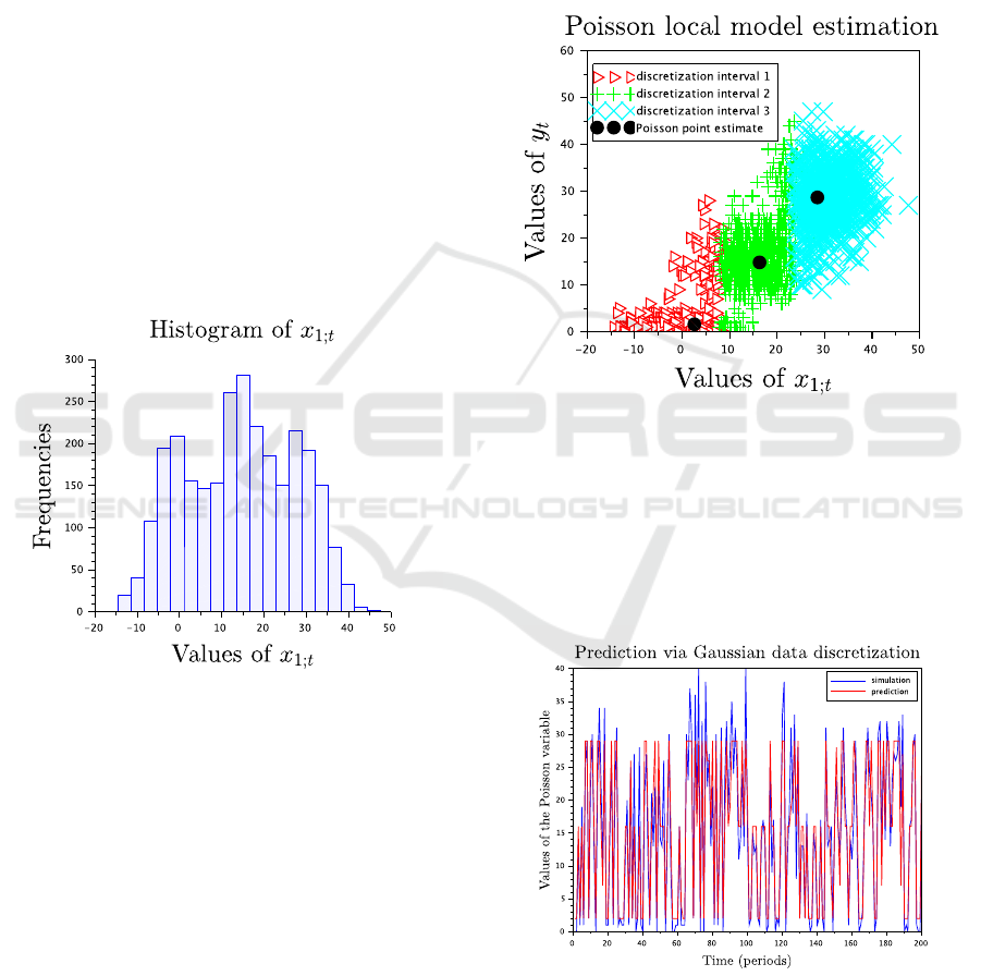
tion intervals. For the illustration, the histogram of

data of one of them used up to the time t = 2800 is

presented in Figure 1.

Figure 1: Histograms of one of the explanatory variable.

Three hills with the centers around -2, 19 and 32

respectively can be guessed in the ﬁgure. These val-

ues are then substituted into the initial statistics V

i;t−1

and indicate the centers of the three clusters for the

discretization part. For the initialization of the counter

statistics κ

i;t−1

, the initial number of data, i.e., the

value of 1, is used for all of the intervals of the vari-

ables.

The expectations of the Gaussian models are esti-

mated using the known ﬁxed variance, which has been

set equal to 5 for all of them. This choice of the vari-

ance value allows to have the clusters of simulated

data partially overlapping, which makes them closer

to reality. The estimation provides twelve discretiza-

tion intervals in the form of clusters located around

their initially guessed and gradually updated centers.

This means that twelve Poisson pdfs are estimated

according to Section 3.2.2 on the obtained intervals

using the data y

measured at the same time instants

as the Gaussian data belonging to the discretized in-

tervals. The illustrative example depicting the XY

graph of the data of the variable x

1;t

and y

is demon-

strated in Figure 2. In this ﬁgure, the point estimates

of the Poisson pdfs obtained locally on each of the

discretization intervals of x

1;t

are denoted by ’•’.

Figure 2: The Poisson local model estimation on the dis-

cretization intervals of the Gaussian variable x

1;t

In the prediction part, the discretization intervals

are determined using the real-time Gaussian data. Us-

ing their proximities, the local Poisson pdfs are united

into the ﬁnal predictive pdf according to Section 3.2.3.

An example of the obtained prediction results is given

in Figure 3.

Figure 3: The Poisson variable prediction using the dis-

cretization of Gaussian explanatory data.

For a comparison, the prediction based on the

Poisson regression described in (Petrou

s et al., 2019)

Prediction of Multimodal Poisson Variable using Discretization of Gaussian Data

605

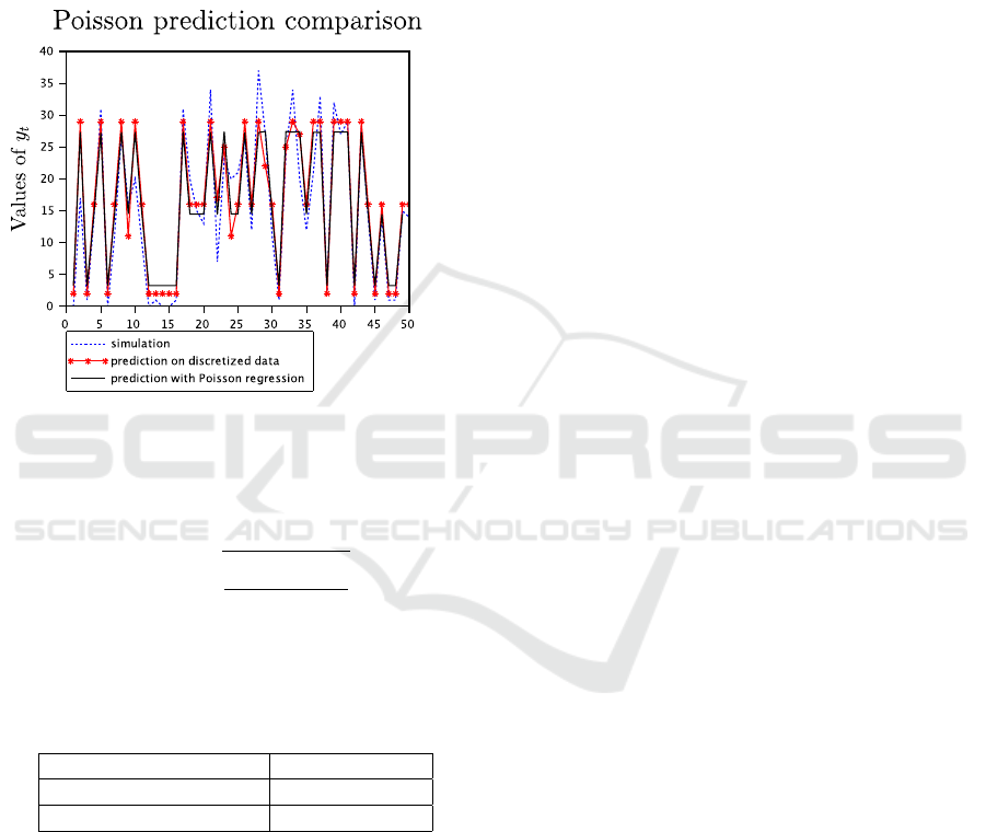
was chosen. The mentioned method includes two

parts: (i) the Poisson mixture model recursive estima-

tion and (i) the least square Poisson regression estima-

tion, which was applied for the prediction of the Pois-

son variable. For this algorithm, the histogram-based

initialization was set for the Poisson components. For

a better visibility, a fragment of the algorithms com-

parison is presented in Figure 4. It can be seen that

the compared results are very close visually.

Figure 4: A fragment of the Poisson variable prediction

based on the discretization of Gaussian explanatory data

compared with the Poisson regression.

To evaluate the prediction accuracy for 200 tested

data, the root-mean-square error was computed

RMSE =

∑

200

t=1

− ˆy

)

200

, (19)

where ˆy

denotes the prediction at time t. The values

of the RMSE averaged over 100 random simulated

datasets can be seen in Table 1.

Table 1: Average RMSE.

Average RMSE

The proposed approach 0.2838133

The Poisson regression 0.2974521

4.1 Discussion

The main aim of the presented study was to verify the

algorithm of the prediction of the Poisson variable us-

ing real-time continuous data for the estimated mod-

els. The aim was successfully achieved. The predic-

tion results look promising and show slight improve-

ments in the comparison with the Poisson regression

as one of the theoretical counterparts.

To highlight advantages brought by the proposed

approach, it is worth noticing the modeling of the

explanatory variables and estimation of the Poisson

model conditioned by the results of this modeling in

the form of values of the discretized variable. This al-

lows to use available explanatory data for the Poisson

prediction in real time recursively, unlike the Poisson

regression estimating the entire explanatory data set

ofﬂine. The use of the individual prior knowledge for

the initialization of the algorithm is another signiﬁ-

cant beneﬁt.

The potential application of the proposed predic-

tion approach can be expected in the area of trans-

portation passenger demand modeling.

The limitations of the approach are concerned

with the assumption of the data multimodality nec-

essary for the discretization with the help of the mix-

ture based clustering as well as using the reproducible

statistics of the involved pdfs.

5 CONCLUSIONS

The presented paper focused on the task of predict-

ing a discrete target variable described by the Pois-

son distribution based on the discretized Gaussian ex-

planatory multimodal data. For the discretization, the

recursive mixture-based clustering algorithms under

Bayesian methodology was used. The Poisson and

Gaussian models were estimated on each of the dis-

cretization intervals using available data in order to

construct the predictive Poisson model, which is used

online for the prediction based on the real-time Gaus-

sian data. The prediction results compared with the

Poisson regression demonstrated minor improving in

the prediction accuracy.

The future work regarding the testing of the al-

gorithm will include (i) experiments with real data,

(ii) setting the higher numbers of the discretization

intervals, which would help not to loss the informa-

tion during the discretization, as well as (iii) setting

the different numbers of the intervals corresponding

to different explanatory variables. The case studies

with other continuous distributions will be also ex-

plored.

ACKNOWLEDGEMENTS

This work was supported by the project Arrowhead

Tools, the project number ECSEL 826452 and MSMT

8A19009.

ICINCO 2021 - 18th International Conference on Informatics in Control, Automation and Robotics

606

REFERENCES

Agresti, A., (2012). Categorical Data Analysis. 3rd Ed. John

Wiley & Sons.

Agresti, A., (2018). An Introduction to Categorical Data

Analysis. 3rd Ed. Wiley, 2018.

Anderson, D. R., Sweeney, D. J., Williams, T. A., Camm,

J. D., Cochran, J. J., (2017). Essentials of Modern

Business Statistics with Microsoft Ofﬁce Excel (Book

Only) 7th Edition. Cengage Learning.

Armstrong, B.G., Gasparrini, A., Tobias, A., (2014). Condi-

tional Poisson models: a ﬂexible alternative to condi-

tional logistic case cross-over analysis. BMC Medical

Research Methodology, 14:122.

Bejleri, V., Nandram, B., (2018). Bayesian and frequentist

prediction limits for the Poisson distribution. Commu-

nications in Statistics - Theory and Methods, 47:17,

4254-4271.

Congdon, P., (2005). Bayesian Models for Categorical Data.

John Wiley & Sons.

Dash, R., Paramguru, R., Dash, R., (2011). Comparative

analysis of supervised and unsupervised discretization

techniques. International Journal of Advances in Sci-

ence and Technology, 2(3): 29:37.

Diallo, A. O., Diop, A., Dupuy, J.-F., (2018). Analysis of

multinomial counts with joint zero-inﬂation, with an

application to health economics, Journal of Statistical

Planning and Inference, vol. 194, p. 85-105.

Doane, D., Seward, L. (2010). Applied Statistics in Busi-

ness and Economics, 3rd Edition, Mcgraw-Hill.

Donnelly Jr., R., (2019). Business Statistics 3rd Edition,

Pearson.

Falissard, B., (2012). Analysis of Questionnaire Data with

R. Chapman & Hall/CRC, Boca Raton.

Forsyth, D., (2019). Applied Machine Learning. Springer.

Gelman, A., Carlin, J. B., Stern, H. S., Dunson, D. B., Ve-

htari, A., Rubin, D. B., (2013). Bayesian Data Ana-

lysis (Chapman & Hall/CRC Texts in Statistical Sci-

ence), 3rd ed., Chapman and Hall/CRC.

Guenni L.B., (2011). Poisson Distribution and Its Appli-

cation in Statistics. In: Lovric M. (eds) International

Encyclopedia of Statistical Science. Springer, Berlin,

Heidelberg. https://doi.org/10.1007/978-3-642-

04898-2 448

Gupta, A., Mehrotra, K., Mohan, C. K., (2010). A

clustering-based discretization for supervised learn-

ing. Statistics & Probability Letters, 80(9-10): 816-

824.

Gupta, M. R. and Chen, Y., (2011). Theory and Use of

the EM Method. (Foundations and Trends(r) in Sig-

nal Processing). Now Publishers Inc.

Heeringa, S.G., West, B.T., Berglung, P.A., (2010). Applied

Survey Data Analysis. Chapman & Hall/CRC.

Jaggia, S., Kelly, A., (2018). Business Statistics: Communi-

cating with Numbers. 3rd Edition. McGraw-Hill Edu-

cation.

Jozov

S., Uglickich, E., Nagy, I., (2021). Bayesian mix-

ture estimation without tears. In: Proceedings of the

18th International Conference on Informatics in Con-

trol, Automation and Robotics (ICINCO 2021), ac-

cepted.

arn

y, M., B

ohm, J., Guy, T.V., Jirsa, L., Nagy, I., Nedoma,

P., Tesa

r, L., (2006). Optimized Bayesian Dynamic

Advising: Theory and Algorithms. Springer, London.

arn

y, M., Kadlec, J., Sutanto, E.L., (1998). Quasi-Bayes

estimation applied to normal mixture. Preprints of the

3rd European IEEE Workshop on Computer-Intensive

Methods in Control and Data Processing, Eds: J.

Roj

cek, M. Vale

ckov

a, M. K

arn

y, K. Warwick, p. 77–

82, CMP ’98 /3./, Prague, CZ, 07.09.1998–09.09.

Kianmehr, K., Alshalalfa, M., Alhajj, R., (2010). Fuzzy

clustering-based discretization for gene expression

classiﬁcation. Knowledge and Information Systems,

vol. 24, 441-465.

Levine, D. M., Stephan, D.F., Krehbiel, T.C., Berenson,

M.L., (2011). Statistics for Managers Using Microsoft

Excel, Sixth Edition. Boston, MA: Prentice Hall.

Li, Y., Sha, Y., Zhao, R., (2010). Poisson prediction of the

loss of teachers in high schools. In: Proceedings of

2010 International Conference on Multimedia Tech-

nology, Ningbo, China, pp. 1-3.

Lim, H. K., Li, W. K., Yu, P. L.H., (2014). Zero-inﬂated

Poisson regression mixture model, Computational

Statistics & Data Analysis, vol. 71, p. 151-158.

Long, J. S., Freese, J., (2014). Regression Models for Cat-

egorical Dependent Variables Using Stata. 3rd Ed.

Stata Press.

Nagy, I., Suzdaleva, E., 2017. Algorithms and Programs

of Dynamic Mixture Estimation. Uniﬁed Approach

to Different Types of Components, SpringerBriefs in

Statistics. Springer International Publishing, 2017.

Nagy, I., Suzdaleva, E., K

arn

y, M., Mlyn

rov

a, T., (2011).

Bayesian estimation of dynamic ﬁnite mixtures. Inter-

national Journal of Adaptive Control and Signal Pro-

cessing. 25(9): 765-787.

Nagy, I., Suzdaleva, E. and Pecherkov

a, P., (2016). Com-

parison of various deﬁnitions of proximity in mix-

ture estimation. In: Proceedings of the 13th Interna-

tional Conference on Informatics in Control, Automa-

tion and Robotics (ICINCO 2016), pp. 527-534.

Perrakis, K., Karlis, D., Cools, M., Janssens, D.,

(2015). Bayesian inference for transportation origin-

destination matrices: the Poisson-inverse Gaussian

and other Poisson mixtures. Journal of the Royal Sta-

tistical Society: Series A (Statistics in Society), vol.

178, p. 271-296.

Peterka, V., (1981). Bayesian system identiﬁcation, in

Eykhoff, P. (Ed.), Trends and Progress in System Iden-

tiﬁcation. Oxford, Pergamon Press, pp. 239-304.

Petrou

s, M., Suzdaleva, E., Nagy, I., (2019). Modeling of

passenger demand using mixture of Poisson compo-

nents. In: Proceedings of the 16th International Con-

ference on Informatics in Control, Automation and

Robotics (ICINCO 2019), p. 617-624.

Petrou

s, M. and Uglickich, E., (2020). Modeling of mixed

data for Poisson prediction. In: Proceedings of IEEE

14th International Symposium on Applied Computa-

Prediction of Multimodal Poisson Variable using Discretization of Gaussian Data

607

tional Intelligence and Informatics (SACI 2020), p.

77-82.

ca, N., Jevti

c, P., McNicholas, P. D., Miljkovic, T.,

(2020). Modeling frequency and severity of claims

with the zero-inﬂated generalized cluster-weighted

models. Insurance: Mathematics and Economics, vol.

94, p. 79-93.

Silva, A., Rothstein, S.J., McNicholas, P.D., Subedi, S.,

(2019). A multivariate Poisson-log normal mixture

model for clustering transcriptome sequencing data.

BMC Bioinformatics 20, 394.

Sinharay, S., (2010). Discrete Probability Distributions. In:

International Encyclopedia of Education. 3rd Edition),

Editor(s): P. Peterson, E. Baker, B. McGaw, Elsevier,

pp.132-134.

Sriwanna, K., Boongoen, T., Iam-On, N., (2019). Graph

clustering-based discretization approach to microar-

ray data. Knowledge and Information Systems, vol.

60, 879-906.

Tang, W., He, H., Tu, X. M., (2012). Applied Categorical

and Count Data Analysis. Chapman and Hall/CRC,

2012.

Yu, J., Gwak, J., Jeon, M., (2016). Gaussian-Poisson mix-

ture model for anomaly detection of crowd behaviour.

In: Proceedings of 2016 International Conference on

Control, Automation and Information Sciences (IC-

CAIS), pp. 106-111.

Zha, L., Lord, D., Zou, Y., (2016). The Poisson inverse

Gaussian (PIG) generalized linear regression model

for analyzing motor vehicle crash data. Journal of

Transportation Safety & Security, vol. 8, p. 18-35.

APPENDIX

Using the na

ıve Bayes principle (Forsyth, 2019)

and the assumption of the independence of the mea-

sured random variables x

and x

, it holds

f (y|x

, x

) ∝ f (x

, x

|y) f (y)

= f (x

|y) f (x

|y) f (y). (20)

According to the Bayes rule, it can be written

f (x

|y) =

f (y|x

) f (x

)

f (y)

, (21)

f (x

|y) =

f (y|x

) f (x

)

f (y)

. (22)

Substituting (21) and (22) into (20), it is obtained

f (y|x

, x

) ∝

f (y|x

) f (x

)

f (y)

f (y|x

) f (x

)

f (y)

f (y|x

) f (x

) f (y|x

) f (x

)

f (y)

f (y|x

) f (y|x

)

f (y)

f (x

) f (x

), (23)

where f (x

) f (x

) is a constant value for the measured

data items x

and x

ICINCO 2021 - 18th International Conference on Informatics in Control, Automation and Robotics

608