Robustness of Contraction Metrics Computed by Radial Basis Functions
Peter Giesl
1 a
, Sigurdur Hafstein
2 b
and Iman Mehrabinezhad
2 c
1
Department of Mathematics, University of Sussex, Falmer BN1 9QH, U.K.
2
Faculty of Physical Sciences, University of Iceland, Dunhagi 5, IS-107 Reykjavik, Iceland
Keywords:
Contraction Metric, Radial Basis Functions, Periodic Orbits, Dynamical System.
Abstract:
We study contraction metrics computed for dynamical systems with periodic orbits using generalized interpo-
lation with radial basis functions. The robustness of the metric with respect to perturbations of the system is
proved and demonstrated for two examples from the literature.
1 INTRODUCTION
Consider an autonomous ordinary differential equa-
tion (ODE) of the form
˙
x = f(x), x ∈ R
n
(1)
with a C
s
-vector field f : R
n
→ R
n
with s ≥ 1. The ex-
istence, uniqueness, and stability of periodic orbits in
a given area can be investigated using a Riemannian
contraction metric. Further, their basins of attraction
can be rigourously estimated. A contraction metric is
a local criterion that does not require knowledge of
the precise location of the periodic orbit and it is ro-
bust to small perturbations of the system. This means
that a contraction metric for (1) remains a contraction
metric for a perturbed system, even with a perturbed
periodic orbit.
A contraction metric provides a local criterion to
compare the evolution of two trajectories – this idea is
also used for the related notions of incremental stabil-
ity, i.e. the stability between two adjacent solutions,
and convergent systems, i.e. systems converging to a
unique solution as time tends to infinity. For a detailed
comparison of these notions, also in non-autonomous
systems, see (R
¨
uffer et al., 2013) and (Fromion and
Scorletti, 2005). Incremental stability was studied
in (Lohmiller and Slotine, 1998) and (Angeli, 2002).
The related notion of Finsler-Lyapunov functions was
introduced by (Forni and Sepulchre, 2014). The study
of contraction metrics in general goes back to (Lewis,
1949; Opial, 1960; Demidovi
ˇ
c, 1961; Demidovi
ˇ
c,
a
https://orcid.org/0000-0003-1421-6980
b
https://orcid.org/0000-0003-0073-2765
c
https://orcid.org/0000-0002-6346-9901
1967). The review (Jouffroy, 2005) puts the defini-
tion from (Lohmiller and Slotine, 1998) into histori-
cal context.
Contraction metrics for periodic orbits have been
considered by (Borg, 1960) with the Euclidean met-
ric and (Stenstr
¨
om, 1962) with a general Riemannian
metric. They have also been studied in (Hartman
and Olech, 1962; Hartman, 1964; Krasovski
˘
i, 1963;
Kravchuk et al., 1992; Leonov et al., 1996).
For periodic orbits, the notions of Zhukovskii sta-
bility, see e.g. (Leonov et al., 2001), i.e. stability of
solutions after reparameterisation of time, has been
used to study stability. The reparameterisation or
synchronisation of the time of adjacent trajectories is
used to show that the existence of a contraction metric
implies the existence of a unique, exponentially sta-
ble periodic orbit to which all trajectories converge,
see (Yang, 2001) or (Manchester and Slotine, 2014).
Converse theorems to prove the existence of a Rie-
mannian contraction metric for a system with an ex-
ponentially stable periodic orbit go back to (Hauser
and Chung, 1994), where a local version is proved,
and (Manchester and Slotine, 2014), where a global
version on a compact sets is proved. The latter also
discusses the robustness to parameters, using the con-
struction in (Leonov, 2006).
(Giesl, 2020) contains a global converse theorem,
showing the existence of a contraction metric on the
entire phase space for systems with an exponentially
stable periodic orbit. The metric was characterized
as the solution of a linear matrix-valued PDE and an
existence and uniqueness theorem was proved. In
(Giesl, 2019) a numerical method using generalized
interpolation with radial basis functions (RBFs) to
compute such a contraction metric was presented. In
592
Giesl, P., Hafstein, S. and Mehrabinezhad, I.
Robustness of Contraction Metrics Computed by Radial Basis Functions.
DOI: 10.5220/0010572905920599
In Proceedings of the 18th International Conference on Informatics in Control, Automation and Robotics (ICINCO 2021), pages 592-599
ISBN: 978-989-758-522-7
Copyright
c
 2021 by SCITEPRESS – Science and Technology Publications, Lda. All r ights reserved

(Giesl et al., 2021b) we presented a rigorous verifica-
tion of the properties of a contraction metric for the
metric computed in (Giesl, 2019) and showed that the
combination delivers a method that is able to compute
and verify a contraction metric for any system with
an exponentially stable periodic orbit. In this paper,
we focus on a perturbation of the system and its effect
with respect to the construction and verification of the
contraction metric computed by our method. Finally,
we present two examples to illustrate the theoretical
result.
The main idea of the procedure in (Giesl et al.,
2021b) is similar to (Giesl et al., 2021a), in which we
provided a computation and verification method for
contraction metrics in the case of exponentially sta-
ble equilibria. As in (Giesl et al., 2021a) we showed
that the method is successful in computing a metric if
sufficiently many collocation points are used in the
computation in (Giesl, 2019) and sufficiently small
simplices in the verification. However, in contrast
to the case of an equilibrium, the contraction condi-
tion for periodic orbits involves the restriction to the
(n −1)-dimensional subspace perpendicular to f(x) at
each point x, which required a more sophisticated ar-
gumentation.
Computational methods for contraction metrics
have been proposed in (Giesl and Hafstein, 2013) for
periodic orbits in time-periodic systems, where the
contraction metric was a continuous piecewise affine
(CPA) function and the contraction conditions were
transformed into constraints of a semidefinite opti-
mization problem. In (Manchester and Slotine, 2014,
Theorem 3) a contraction metric for periodic orbits
was constructed using Linear Matrix Inequalities and
SOS (sum of squares). While both of these meth-
ods also include a rigorous verification, similar to our
approach, they are of higher computational complex-
ity because they require solving a semidefinite opti-
mization problem, whereas solving a system of lin-
ear equations is computationally the most demanding
step in the approach from (Giesl et al., 2021b).
2 SUMMARY OF THE METHOD
In this section, we briefly review contraction metrics
for periodic orbits and the method from (Giesl et al.,
2021b); more details on both can be found in (Giesl
et al., 2021b). We first need a few definitions.
Definition 2.1 (Riemannian/contraction metric).
Let G be an open subset of R
n
. A Riemannian
metric is a locally Lipschitz continuous matrix-valued
function M : G → S
n×n
, such that M(x) is positive
definite for all x ∈ G, where S
n×n
denotes the sym-
metric n × n matrices with real entries.
A contraction metric for a periodic orbit is a Rieman-
nian metric M : G → S
n×n
fulfilling a contraction
condition expressed by L
M
(x) ≤ −ν < 0 for all
x ∈ K ⊂ G, where L
M
is defined in (3) below and K
is a compact subset of the open set G ⊂ R
n
such that
f(x) 6= 0 holds for all x ∈ K. For the definition of L
M
we first define for all x ∈ R
n
with f(x) 6= 0
V (x) = Df(x) −
f(x)f(x)
T
(Df(x) + Df(x)
T
)
kf(x)k
2
2
. (2)
For all x ∈ R
n
with f(x) 6= 0 we define
(3)
L
M
(x) = max
v∈R
n
,v
T
M(x)v=1,v
T
f(x)=0
L
M
(x;v) where
L
M
(x;v) =
1
2
v
T

M
0
+
(x) +V (x)
T
M(x) + M(x)V (x)

v.
The forward orbital derivative M
0
+
(x) with respect to
(1) at x ∈ G is defined by
M
0
+
(x) := limsup
h→0
+
M

S
h
x

− M(x)
h
(4)
where t 7→ S
t
x is the solution to (1) passing through
x at time t = 0. We refer to M as a (Riemannian)
contraction metric on K or a metric contracting in K.
The function L
M
(x;v) in (3) above is negative for
v with v
T
f(x) = 0, if for small δ > 0 the distance be-
tween solutions through x and x + δv decreases with
respect to the metric M(x). For a heuristic explana-
tion of this fact, see, e.g. (Giesl, 2019, Section 1).
Two theorems reveal the connection between pe-
riodic orbits and contraction metrics. (Giesl et al.,
2021b, Theorem 2.5) shows that the existence of a
contraction metric on a compact, forward invariant set
K asserts the existence of a unique exponentially sta-
ble periodic orbit Ω ⊂ K and that K is a subset of the
orbit’s basin of attraction, i.e. K ⊂ A(Ω). Conversely,
(Giesl, 2020, Theorems 3.1, 4.2) establish the exis-
tence of a contraction metric for exponentially sta-
ble periodic orbits, as the solution to a matrix-valued
PDE. In order to explain this in more detail, we first
need to define for all x ∈ R
n
with f(x) 6= 0 the linear
differential operator L, acting on M ∈ C
0
(R
n
;S
n×n
)
by
LM(x) := M
0
+
(x) +V (x)
T
M(x) + M(x)V (x), (5)
where V was defined in (2). Moreover, we define the
projection P
x
for all x ∈ R
n
with f(x) 6= 0 onto the
(n − 1)-dimensional space perpendicular to f(x), i.e.
P
2
x
= P
x
, P
x
f(x) = 0 and P
x
v = v if v
T
f(x) = 0, by
P
x
:= I
n×n
−
f(x)f(x)
T
kf(x)k
2
2
. (6)
Robustness of Contraction Metrics Computed by Radial Basis Functions
593

Then for B ∈ C
s−1
(A(Ω);S
n×n
) such that B(x)
is positive definite for all x ∈ A(Ω), we define C ∈
C
s−1
(A(Ω);S
n×n
) by
C(x) = P
T
x
B(x)P
x
. (7)
(Giesl, 2020, Theorems 3.1 and 4.2) assert that there
exists a unique solution M ∈ C
s−1
(A(Ω);S
n×n
) of the
linear matrix-valued PDE
LM(x) = −C(x) for all x ∈ A(Ω) (8)
satisfying f(x
0
)
T
M(x
0
)f(x
0
) = c
0
kf(x
0
)k
4
2
, (9)
where x
0
∈ A(Ω) and c
0
∈ R
+
are fixed. The
first step of the method in (Giesl et al., 2021b) to
rigorously compute a contraction metric is to follow
(Giesl, 2020) and solve the PDE (8) numerically
using RBFs to obtain a contraction metric that can
be computed knowing the values LM(x
i
) at finitely
many collocation points x
i
within a set O. This
procedure is referred to as a generalized interpolation
problem or the optimal recovery problem, because it
produces a function S fulfilling LS(x
i
) that is norm
minimal in the corresponding reproducing kernel
Hilbert space (RKHS). The existence and uniqueness
of the optimal recovery has been proved in (Giesl,
2019, Theorem 4.2) and error estimates for the RBF
approximation have been obtained in (Giesl, 2019,
Theorem 4.4). While this theorem provides a proof
that the RBF approximation S to M is a contraction
metric if the so-called fill distance h
X,O
of the set of
collocation points X in O is small enough, it does
not quantify in a useful way how small h
X,O
must be
because unknown constants appear in the estimate.
This is why we need a verification method that allows
us to check whether S is a contraction metric or
whether we need add collocation points to make h
X,O
smaller.
Thus, in the second step of the method from (Giesl
et al., 2021b) the conditions for a contraction metric
are rigorously verified for the CPA interpolation P
of the contraction metric S, which was computed in
the first step. In particular, it is verified that P(x) is
positive definite and L
P
(x) is negative definite for
all x ∈ D
◦
T
, see (Giesl et al., 2021b, Theorem 4.11),
where D
T
is the area triangulated by the triangulation
T . In (Giesl et al., 2021b) error estimates and
statements about the CPA interpolation are provided,
together with criteria that assert that the interpolation
is a contraction metric itself. The essential point is
that these criteria can be verified numerically very
efficiently.
To be more precise, given a system
˙
x = f(x), f ∈
C
3
(R
n
;R
n
), and a finite triangulation T =
S
ν
S
ν
of
D
T
⊂ R
n
with vertex set x
k
∈ V
T
, such that f(x) 6=
0 for all x ∈ D
T
, we need the check the following
constraints:
(VP1) Positive definiteness of P
For each vertex x
k
∈ V
T
P(x
k
) is positive def-
inite, i.e. :
P(x
k
)  0
n,n
.
(VP2) Negative definiteness of A
ν
− κ
∗
ν
ff
T
For each simplex S
ν
= co(x
0
, . . . , x
n
) ∈ T
(convex hull) and each vertex x
k
of S
ν
:
A
ν
(x
k
) − κ
∗
ν
f(x
k
)f
T
(x
k
) + h
2
ν
E
ν
I
n×n
≺ 0
n,n
.
Here
A
ν
(x
k
) := P(x
k
)V (x
k
) +V (x
k
)
T
P(x
k
) +

∇P
ν
i j
· f(x
k
)

i, j=1,2,...,n
, (10)
where κ
∗
ν
, and E
ν
are tailored constants for the
system for each simplex S
ν
∈ T , and h
ν
is its
diameter h
ν
:= diam(S
ν
) = max
x,y∈S
ν
kx −
yk
2
.
Our verification problem is a semidefinite feasibil-
ity problem and can in theory be solved as such. How-
ever, it is computationally much more efficient to as-
sign values to the variables P(x
k
) of the problem using
the optimal recovery S of the solution to (8) and (9),
i.e. P(x
k
) = S(x
k
), and then verify that the constraints
of the feasibility problem are fulfilled. We will refer
to this feasibility problem as verification problem. A
contraction metric M for the system (1) will also be
a contraction metric for a perturbed system, as shown
in the next theorem. To quantify perturbations we de-
fine for W ∈ C
k
(D; R ), where D ⊂ R
n
is a non-empty
open set and R is R, R
n
, S
n×n
, or R
n×n
, the C
k
-norm
as
k
W
k
C
k
(D;R )
:=
∑
|α|≤k
sup
x∈D
k
D
α
W (x)
k
2
.
In this formula α ∈ N
n
0
is a multi-index and |α| =
∑
n
i=1
α
i
.
Theorem 2.2. Assume that M : G → S
n×n
is a con-
traction metric as in Definition 2.1 for system (1),
where f is C
1
, and contracting in the compact set
K ⊂ G. Then there is an ε > 0 such that M : G → S
n×n
is also a contraction metric for any perturbed system
˙
x =
e
f(x), where
e
f is C
1
and k
e
f − fk
C
1
(G;R
n
)
< ε.
Proof. By assumption M(x) is symmetric and posi-
tive definite for every x ∈ G ⊂ R
n
. Hence, we only
need to verify that L
M
(x) < 0 holds true for all x ∈ K
when f has been substituted by
e
f in (2), (3), and (4).
We choose ε > 0 so small that
e
f(x) 6= 0 for all
x ∈ K. Then we note, that the right-hand side of
formula (2) is a continuous function of y = f(x) and
Z = Df(x). Thus V (x) varies continuously when f
is substituted by
e
f with k
e
f − fk
C
1
(G;R
n
)
< ε. To see
ICINCO 2021 - 18th International Conference on Informatics in Control, Automation and Robotics
594

that (4) varies continuously we recall standard results
on the continuous dependence of solutions to ODE,
e.g. (Walter, 1998, §12.V), which implies that from
k
e
f − fk
C
1
(G;R
n
)
< ε follows
k
e
S
h
x − S
h
xk
2
≤
ε
L
(e
Lh
− 1),
where S
h
x and
e
S
h
x are the solutions at time h > 0,
starting at x ∈ K to
˙
x = f(x) and
˙
x =
e
f(x) respectively,
and the solution trajectories are in an open set O, K ⊂
O ⊂ O ⊂ G, and O is compact. Further, 0 < L < ∞ is
a Lipschitz constant for f in O.
Let 0 < L
∗
< ∞ be a Lipschitz constant for M on O
with respect to the k · k
2
norm. Then we have





M(
e
S
h
x) − M(x)
h
−
M(S
h
x) − M(x)
h





2
=
L
∗
h
k
e
S
h
x − S
h
xk
2
≤ L
∗
ε
e
Lh
− 1
Lh
≤ 2L
∗
ε
for small enough h > 0. Thus M
0
+
(x) also varies
continuously when f is substituted by
e
f with k
e
f −
fk
C
1
(G;R
n
)
< ε and we have established that L
M
(x;v)
varies continuously. The assertion now follows from
the fact that both the argument of the maximum in (3)
and the set maximized over, an intersection of an el-
lipsoid with a hyper-plane, vary continuously when f
is substituted by
e
f with k
e
f − fk
C
1
(G;R
n
)
< ε, because
neither f(x) = 0 nor
e
f(x) = 0 on K. Thus L
M
(x) < 0
remains true after the substitution if ε > 0 is small
enough.
This robustness property is a very desired property
in dynamical systems. Note also that one could even
prove that (VP1) and (VP2) of the verification remain
true after a small perturbation, but then one must de-
mand that f,
e
f are C
3
and that k
e
f − fk
C
2
(G;R
n
)
< ε be-
cause the constants E
ν
in (VP2) depend on the second
derivatives of the right-hand side of the system (1).
A short discussion of the numerical complexity
of our method follows: The number of elementary
arithmetic operations needed for computing the co-
efficients of the collocation matrix in the RBF-step
is of the order O(N
2
) for a fixed n, where N is the
number of collocation points and n is the dimension
of the system. The order in n for a fixed N is at least
O(n
5
); depending on f and D f it might be higher. To
solve the linear equations O((Nn
2
)
3
) = O(N
3
n
6
) ele-
mentary operations are needed. Typically N  n and
therefore the complexity of the first step of the algo-
rithm is O(N
3
n
6
), where we consider the dimension n
of the system to be fixed.
In the second step of the method, we first evalu-
ate P(·) at every vertex of the triangulation. For each
vertex we need O(N) elementary operations for this,
again ignoring the dependance on n. Then we verify
the constraints (VP1)-(VP2). Since this must be done
for every vertex we need at least O(N
CPA
N) opera-
tions, where N
CPA
denotes the number of vertices of
the triangulation.
Clearly, the number of simplices in the triangula-
tion is bounded above by N
CPA
n!. Therefore, the com-
plexity of the verification of the constraints (VP1)-
(VP2) is linear in N
CPA
and independent of N. Thus,
the numerical complexity of the second step of the
method is O(N
CPA
N), again assuming a fixed dimen-
sion n. However, note that the computational effort
grows very fast with the dimension n of the system,
in particular since N and N
CPA
can be expected to
grow exponentially with the dimension (curse of di-
mensionality).
In the next section we demonstrate the applicabil-
ity of our theoretical results to two examples. Note
that the periodic orbit is displayed in the figures
through a numerical approximation for comparison in
orange, but the method verifies rigorously that it ex-
ists and is exponentially stable and, moreover, deter-
mines a subset of its basin of attraction.
3 EXAMPLES
We implemented our method in C++ and ran the ex-
amples on an AMD Ryzen 2700X processor with 8
cores at 3.7 GHz and with 64GB RAM. In order to
compute a positively invariant set K for the dynam-
ical systems
˙
x = f(x) we use a procedure motivated
by (Giesl and Hafstein, 2015). First we solve numer-
ically the PDE
n
∑
i=1
∂V
∂x
i
(x) f
i
(x) = ∇V (x) · f(x)
= −
q
δ
2
+ kf(x)k
2
2
, (11)
with δ = 10
−8
, using RBF. Then we use CPA interpo-
lation V
P
of the numerical solution and verify where
∇V
P
(x) · f(x) < 0 holds true. In this area the func-
tion V
P
is decreasing along solution trajectories and a
sublevel set {x ∈ R
n
: V
P
(x) ≤ c} is necessarily for-
ward invariant, if its boundary is fully contained in
this area. Hence, we only need ∇V
P
(x) · f(x) < 0 on
the level set {x ∈ R
n
: V
P
(x) = c}, not on the whole
sublevel set. We refer to V
P
as Lyapunov-like func-
tion.
The failing points of the Lyapunov-like function (see
for example Figure 2) are the points where the func-
tion V
P
is not decreasing along solution trajectories.
In order to obtain a positively invariant set, we need to
Robustness of Contraction Metrics Computed by Radial Basis Functions
595

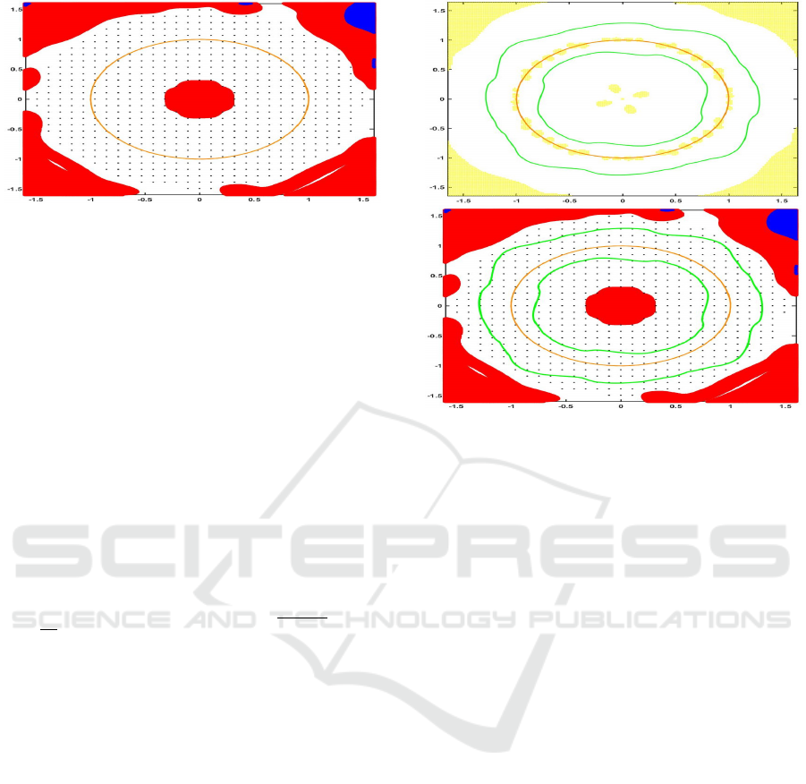
Figure 1: Example 3.1. The black dots show the collocation
points and the orange curve is the periodic orbit for system
(12). We plot the area where the constraints of Verifica-
tion Problem fail to be fulfilled; in blue if (VP1) is violated
and in red if (VP2) is violated. Where neither is violated
(white), the CPA interpolation P fulfills the properties of a
contraction metric.
find a sublevel set of the function such that its bound-
ary does contain any of these points.
3.1 Unit Circle
As a first example, we consider the following system

˙x = x(1 − x
2
− y
2
) − y
˙y = y(1 − x
2
− y
2
) + x
(12)
of which the unit circle is an exponentially stable pe-
riodic orbit and the origin is an unstable equilibrium.
We choose B(x) = I
2×2
and the collocation points
X =
1.6
15
Z
2
∩ {(x, y) ∈ R
2
: 0.25 <
p
x
2
+ y
2
< 1.5}
as well as the point x
0
= (1, 0) with c
0
= 1. We
use a kernel φ(x, y) = ψ
6,4
(kx − yk
2
) given by the
Wendland function ψ
6,4
(r) = (1 − r)
10
+
[25 + 250r +
1, 050r
2
+2, 250r
3
+2, 145r
4
] where x
+
= x for x ≥ 0
and x
+
= 0 for x < 0. The corresponding Sobolev
space is H
5.5
(R
2
;S
2×2
). The grid X has N = 600
collocation points, black dots in Figure 1. We mark
the area where the constraints of Verification Prob-
lem fail to be fulfilled; in blue if (VP1) is violated
and in red if (VP2) is violated. We used the stan-
dard triangulation, cf. (Giesl and Hafstein, 2015), of
the area [−1.6, 1.6] × [−1.6, 1.6] with 1500
2
vertices
for the CPA interpolation. In order to obtain a pos-
itively invariant set, we computed a Lyapunov-like
function solving (11) using RBF and interpolating the
solution with a CPA interpolation. We used the same
collocation grid X, but another Wendland function
ψ
5,3
(cr) with parameter c = 0.9 and a triangulation
of [−1.65, 1.65] × [−1.65, 1.65] with 1000
2
vertices.
In the first plot of Figure 2, the failing points for the
Lyapunov-like function are marked in yellow and the
level set is the curve in green. The periodic orbit is
the curve in orange. In the second figure, the level set
Figure 2: Example 3.1. The orange curve indicates the pe-
riodic orbit for system (12). The yellow areas denote the
simplices, where the Lyapunov-like function is not decreas-
ing. The green curves are the level set of the Lyapunov-like
function, which thus indicate the boundary of a positively
invariant set. The second figure shows the positively in-
variant set (bounded by the green curves), the collocation
points (black dots) as well as the blue area, where (VP1) is
not fulfilled, and the red area, where (VP2) is not satisfied.
The positively invariant set (bounded by the green curves) is
thus a subset of the basin of attraction of a unique periodic
orbit within it.
of the Lyapunov-like function and the area suggested
by our method suitable for the contraction metric are
displayed together. Thus, the sublevel set is a subset
of the basin of attraction of a unique periodic orbit.
We now consider the perturbed system

˙x = (x + ε)(1 − x
2
− y
2
) − (y + ε)
˙y = (y + ε)(1 − x
2
− y
2
) + (x + ε)
(13)
with ε = 0.2. We use the same Lyapunov function and
contraction metric as in the unperturbed system. We
can see in plots of Figure 3 that both the contraction
metric and the Lyapunov-like function computed for
the unperturbed system satisfy the constraints for the
perturbed system in a very similar area as before.
3.2 A Three-dimensional Example
We consider the following three-dimensional system
from (Giesl, 2019, Section 5.3)



˙x = x(1 − x
2
− y
2
) − y + 0.1yz
˙y = y(1 − x
2
− y
2
) + x
˙z = −z + xy
(14)
ICINCO 2021 - 18th International Conference on Informatics in Control, Automation and Robotics
596

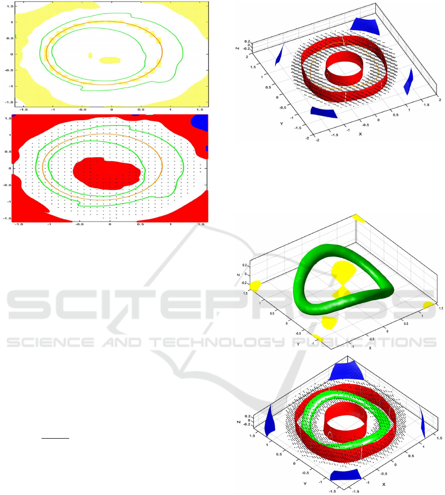
Figure 3: Example 3.1. The orange curve indicates the pe-
riodic orbit of the perturbed system (13) with ε = 0.2. The
yellow areas denote the simplices, where the Lyapunov-like
function is not decreasing. The green curves are the level
set of the Lyapunov-like function, which thus indicate the
boundary of a positively invariant set. The second figure
shows the positively invariant set (green), the collocation
points (black dots) as well as the blue area, where (VP1), is
not fulfilled and the red area, where (VP2) is not satisfied.
The positively invariant set (bounded by the green curves)
is thus a subset of the basin of attraction of a unique peri-
odic orbit within it – note that the contraction metric and
Lyapunov-like function have been computed for the unper-
turbed system, but the conditions are checked for the per-
turbed system.
which has an exponentially stable periodic orbit.
We choose the parameters of the method in the
following way: B(x) = I
3×3
and N = 4, 458 col-
location points to cover the area {(x, y, z) ∈ R
3
:
0.75 <
p
x
2
+ y
2
< 1.55, |z| < 0.45} using a hexag-
onal grid, see (Iske, 1998), and a scaling factor
α = (0.1398, 0.1398, 0.09), as well as the point x
0
=
(1, 0, 0) with c
0
= 1. We use the kernel given by
the Wendland function ψ
6,4
with parameter c = 0.55,
the corresponding Sobolev space is H
6
(R;S
3×3
). In
Figure 4, the black dots are the collocation points,
the orange curve is the periodic orbit, the blue sur-
face represents the boundary of area where (VP1)
is not satisfied and the red surface is the boundary
of area where (VP2) is not fulfilled. We have tri-
angulated the space [−1.67, 1.67] × [−1.67, 1.67] ×
[−0.67, 0.67] with 601
3
vertices.
For the Lyapunov-like function we use the same
set of collocation points, and the kernel given by the
Figure 4: Example 3.2. The orange curve indicates the
periodic orbit for system (14). The black dots show the col-
location points. The blue surface indicates the boundary of
area where (VP1) is not fulfilled. The red surface indicates
the boundary of the area where (VP2) is not satisfied.
Figure 5: Example 3.2. The area where the Lyapunov-
like function, computed for system (14), is not decreasing
is plotted in yellow. The green surface is the level set of the
Lyapunov-like function, which thus indicates the boundary
of a positively invariant set. The second figure shows the
collocation points (black dots) as well as the boundary of
the area where (VP1) is not fulfilled (blue), and the bound-
ary of the area where (VP2) is not satisfied (red). The pos-
itively invariant set (bounded by the green surface in the
middle) is thus a subset of the basin of attraction of a unique
periodic orbit within it.
Robustness of Contraction Metrics Computed by Radial Basis Functions
597

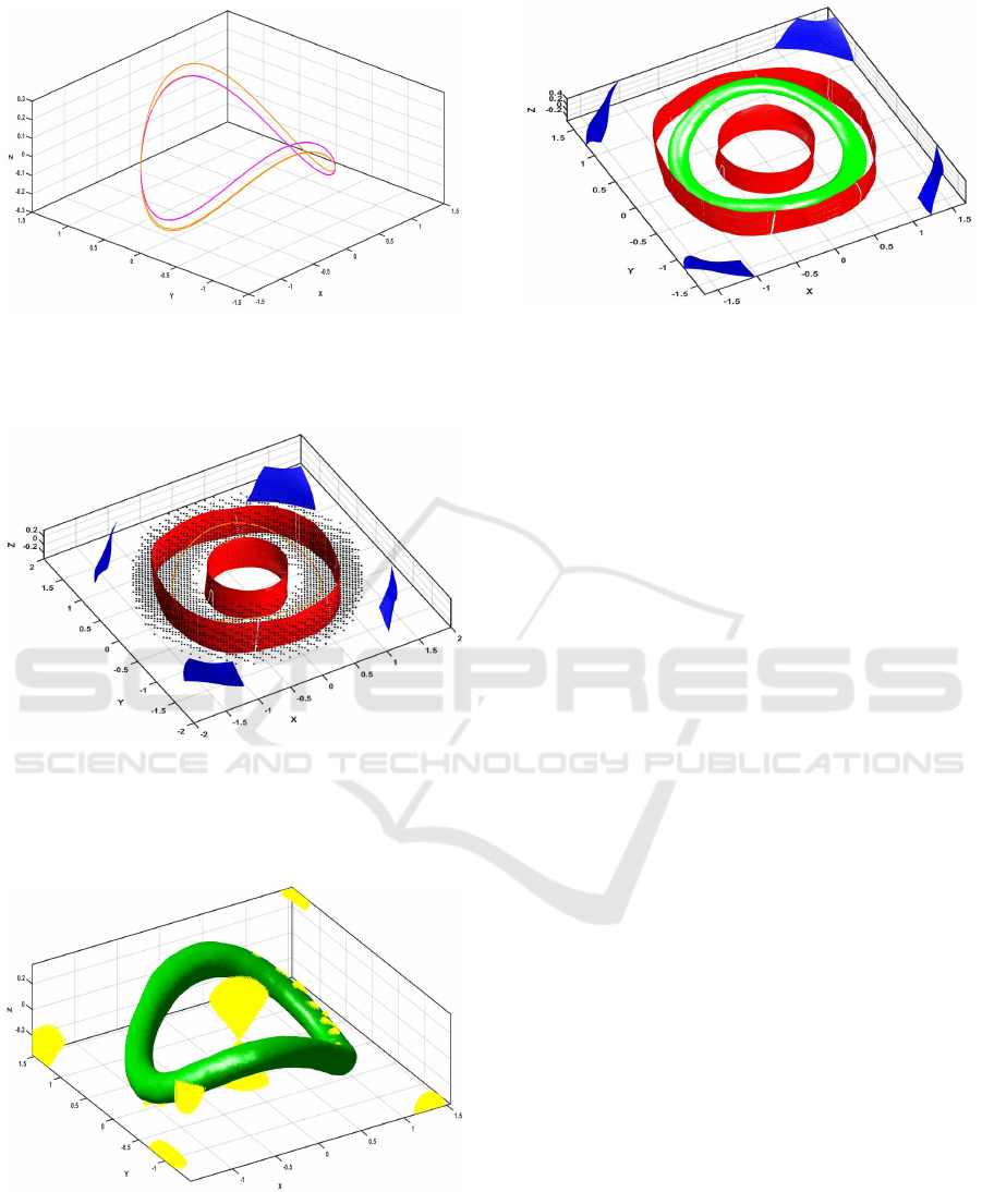
Figure 6: Example 3.2. The periodic orbit for the original
system (14) is the curve in magenta, while the periodic orbit
for the perturbed system (15) with ε = 0.1 is depicted in
orange.
Figure 7: Example 3.2. The contraction metric, computed
for the unperturbed system, is checked for the perturbed
system: the blue surface shows the boundary of the area
where (VP1) fails, while the red surface denote the bound-
ary of the area where (VP2) fails.
Figure 8: Example 3.2.The Lyapunov-like function for the
unperturbed system (14) cannot be used for the perturbed
system (15) with ε = 0.1, because the failing points, where
it is not decreasing along solution trajectories, intersects the
boundary of the level-set (green).
Figure 9: Example 3.2. By computing a new Lyapunov-
like function for the perturbed system (15) with ε = 0.1, we
can verify that the area bounded by the green surface is for-
ward invariant. The contraction metric for the unperturbed
system can still be used; the boundary of the area where
(VP1) is not fulfilled is depicted in blue and the boundary
of the area where (VP2) is not satisfied is drawn in red. The
positively invariant set (bounded by the green surface in the
middle) is thus a subset of the basin of attraction of a unique
periodic orbit within it.
Wendland function ψ
5,3
with parameter c = 0.6. In
Figure 5, a suitable level set of the Lyapunov-like
function is presented in green, while its failing points
are in yellow. The second side figure combines all the
results, showing that the conditions of the verification
problem are satisfied within a compact, and positively
invariant set (green).
Now we consider the perturbed system



˙x = x(1 − x
2
− y
2
) − y + 0.1(y + ε)z
˙y = y(1 − x
2
− y
2
) + x
˙z = −z + x(y + ε)
(15)
with ε = 0.1. The periodic orbist for the original (ma-
genta) and perturbed (orange) systems can be seen in
Figure 6. It is an interesting observation that while
the same contraction metric could be used for the per-
turbed system, see Figure 7, the Lyapunov-like func-
tion fails to give a suitable level set around the peri-
odic orbit and we need to calculate a new one for the
perturbed system, see Figure 8.
4 CONCLUSIONS
A contraction metric can be used to determine a sub-
set of the basin of attraction of a periodic orbit. Hav-
ing a PDE characterization of the contraction metric,
one can use generalized interpolation with radial basis
functions to approximate the solution of the PDE and
thus to compute a contraction metric. Subsequently
the approximation can be interpolated over a triangu-
lation and it can be rigorously verified that the con-
ICINCO 2021 - 18th International Conference on Informatics in Control, Automation and Robotics
598

structed matrix-valued function truly is a contraction
metric.
In this paper it was shown, both in theory and ex-
amples, that the contraction metric has the advantage
of being robust with respect to small perturbations in
the system, even those which vary the position of the
periodic orbit.
When compared to other methods to determine the
basin of attraction of an exponentially stable periodic
orbit, e.g. Lyapunov functions, the computation of a
contraction metric is computationally more demand-
ing as we construct a matrix-valued function. The ad-
vantage is, however, that we do not need the location
of the periodic orbit and that the metric is robust with
respect to perturbations of the system.
REFERENCES
Angeli, D. (2002). A Lyapunov approach to incremen-
tal stability properties. IEEE Trans. Automat. Contr.,
47(3):410–421.
Borg, G. (1960). A condition for the existence of orbitally
stable solutions of dynamical systems, volume 153.
Elander.
Demidovi
ˇ
c, B. P. (1961). On the dissipativity of a certain
non-linear system of differential equations. I. Vestnik
Moskov. Univ. Ser. I Mat. Meh., 1961(6):19–27.
Demidovi
ˇ
c, B. P. (1967). Lekcii po matematiq-
esko˘i teorii usto˘i qivosti. Izdat. “Nauka”,
Moscow.
Forni, F. and Sepulchre, R. (2014). A differential Lyapunov
framework for Contraction Analysis. IEEE Transac-
tions on Automatic Control, 59(3):614–628.
Fromion, V. and Scorletti, G. (2005). Connecting nonlinear
incremental Lyapunov stability with the linearizations
Lyapunov stability. In Proc. 44th IEEE Conf. Decis.
Control, pages 4736–4741.
Giesl, P. (2019). Computation of a contraction metric for
a periodic orbit using meshfree collocation. SIAM J.
Appl. Dyn. Syst., 18(3):1536–1564.
Giesl, P. (2020). On a matrix-valued PDE characterizing a
contraction metric for a periodic orbit. Discrete Con-
tin. Dyn. Syst. Ser. B, accepted.
Giesl, P. and Hafstein, S. (2013). Construction of a CPA
contraction metric for periodic orbits using semidefi-
nite optimization. Nonlinear Anal., 86:114–134.
Giesl, P. and Hafstein, S. (2015). Computation and verifica-
tion of Lyapunov functions. SIAM J. Appl. Dyn. Syst.,
14(4):1663–1698.
Giesl, P., Hafstein, S., and Mehrabinezhad, I. (2021a).
Computation and verification of contraction metrics
for exponentially stable equilibria. J. Comput. Appl.
Math., accepted.
Giesl, P., Hafstein, S., and Mehrabinezhad, I. (2021b).
Computation and verification of contraction metrics
for periodic orbits. J. Math. Anal. Appl., accepted.
Hartman, P. (1964). Ordinary Differential Equations. Wi-
ley, New York.
Hartman, P. and Olech, C. (1962). On global asymptotic
stability of solutions of differential equations. Trans.
Amer. Math. Soc., 104:154–178.
Hauser, J. and Chung, C. C. (1994). Converse Lyapunov
functions for exponentially stable periodic orbits. Sys-
tems Control Lett., 23(1):27–34.
Iske, A. (1998). Perfect centre placement for radial ba-
sis function methods. Technical Report TUM-M9809,
TU Munich, Germany.
Jouffroy, J. (2005). Some ancestors of contraction analysis.
In 44th IEEE Conference on Decision and Control,
page 5450. IEEE.
Krasovski
˘
i, N. N. (1963). Problems of the Theory of Stabil-
ity of Motion. Mir, Moskow, 1959. English translation
by Stanford University Press.
Kravchuk, A. Y., Leonov, G. A., and Ponomarenko, D. V.
(1992). A criterion for the strong orbital stability of
the trajectories of dynamical systems I. Diff. Uravn.,
28:1507–1520.
Leonov, G., Noack, A., and Reitmann, V. (2001). Asymp-
totic orbital stability conditions for flows by estimates
of singular values of the linearization. Nonlinear
Anal., 44(8):1057–1085.
Leonov, G. A. (2006). Generalization of the Andronov-Vitt
theorem. Regul. Chaotic Dyn., 11(2):281–289.
Leonov, G. A., Burkin, I. M., and Shepelyavyi, A. I. (1996).
Frequency Methods in Oscillation Theory. Ser. Math.
and its Appl.: Vol. 357, Kluwer.
Lewis, D. C. (1949). Metric properties of differential equa-
tions. American Journal of Mathematics, 71(2):294–
312.
Lohmiller, W. and Slotine, J.-J. (1998). On Contrac-
tion Analysis for Non-linear Systems. Automatica,
34:683–696.
Manchester, I. R. and Slotine, J.-J. E. (2014). Transverse
contraction criteria for existence, stability, and robust-
ness of a limit cycle. Systems Control Lett., 63:32–38.
Opial, Z. (1960). Sur la stabilit
´
e asymptotique des solutions
d’un syst
`
eme d’
´
equations diff
´
erentielles. Ann. Polon.
Math., 7(3):259–267.
R
¨
uffer, B., van de Wouw, N., and Mueller, M. (2013). Con-
vergent system vs. incremental stability. Systems Con-
trol Lett., 62(3):277–285.
Stenstr
¨
om, B. (1962). Dynamical systems with a certain
local contraction property. Math. Scand., 11:151–155.
Walter, W. (1998). Ordinary Differential Equation.
Springer.
Yang, X. (2001). Remarks on three types of asymptotic
stability. Systems Control Lett., 42:299–302.
Robustness of Contraction Metrics Computed by Radial Basis Functions
599