On a Wireless Sensor Network Problem with Spanning Tree Backbone

Pablo Adasme

1 a

and Ali Dehghan Firoozabadi

2 b

Department of Electrical Engineering, Universidad de Santiago de Chile, Avenida Ecuador 3519, Santiago, Chile

Department of Electricity, Universidad Tecnol

ogica Metropolitana,

Av. Jose Pedro Alessandri 1242, 7800002, Santiago, Chile

Keywords:

Combinatorial Optimization, p-Median and Spanning Tree Problems, Mixed-integer Linear Programming,

Wireless Sensor Networks, Local Search Algorithm.

Abstract:

Let G = (V, E) be a complete graph with set of nodes V = {1, . . . , n} and edge set E = {1, . . . , m} representing

a wireless sensor network. In this paper, we consider the problem of ﬁnding a minimum cost spanning tree

backbone formed with p ∈ Z

out of n nodes where p < n in such a way that the n − p remaining nodes

of G are connected to the leaf nodes of the backbone structure at minimum connectivity cost. Notice that

this problem arises as a combination of two classical combinatorial optimization problems, namely the p-

Median and spanning tree problems. We propose two mixed-integer linear programming (MIP) formulations

for this problem as well as a local search heuristic. The proposed models and algorithm can be used as a

reference source for comparison purposes when designing future network protocols. We consider complete

graph instances with Euclidean and random uniform costs. Our preliminary numerical results indicate that one

of the proposed models performs slightly better than the other one in terms of solution quality and CPU times

obtained with the Gurobi solver. Finally, the proposed heuristic allows one to obtain near-optimal solutions in

remarkably less CPU time compared to the MIP models.

1 INTRODUCTION

The topic of wireless sensor networks has attracted

continuously increased attention by both the research

and industry communities within the last decades.

This is mainly due to the fact that there exists a huge

potential space for application deployments related to

these types of networks. Examples of applications

include environmental observation and forecasting,

disaster prevention, structure health, industrial mon-

itoring, agriculture production, security, and military

surveillance, to name a few (BenSaleh et al., 2020).

Consequently, new technologies are being developed

to support these future network deployments. Optical

wireless communications and massive multiple-input

multiple-output (MIMO) transmission technologies

are examples of 5G and 6G protocols enabling a bet-

ter quality of service for an ever-increasing number

of users (Chowdhury et al., 2020; Huang et al., 2019;

Jiang et al., 2021).

In this paper, we consider an optimization prob-

lem related to the required infrastructure for these

https://orcid.org/0000-0003-2500-3294

https://orcid.org/0000-0002-6391-6863

types of networks. More precisely, let G = (V, E) be a

complete graph with set of nodes V = {1, . . . , n} and

edge set E = {1, . . . , m} representing a wireless sen-

sor network. We consider the problem of ﬁnding a

minimum cost spanning tree backbone formed with

p ∈ Z

out of n nodes where p < n in such a way

that the n − p remaining nodes of G are connected to

the leaf nodes of the backbone structure at minimum

connectivity cost. Notice that this problem arises as a

combination of two classical combinatorial optimiza-

tion problems, namely the p-Median and spanning

tree problems. We propose two mixed-integer pro-

gramming (MIP) formulations for this problem and

a local search heuristic that allows obtaining near-

optimal solutions in signiﬁcantly shorter CPU time

when compared to the MIP models. Our ﬁrst model

is formulated based on a Miller-Tucker-Zemlin con-

strained approach. Whereas the second one is a sin-

gle ﬂow-based formulation (Adasme, 2018; Adasme

et al., 2018; Adasme, 2019; Adasme et al., 2017). No-

tice that in principle, the proposed models allow ob-

taining the optimal solution of the problem and hence

they can be used as a reference source for compar-

ison purposes when designing future network proto-

Adasme, P. and Firoozabadi, A.

On a Wireless Sensor Network Problem with Spanning Tree Backbone.

DOI: 10.5220/0010569700760082

In Proceedings of the 18th International Conference on Wireless Networks and Mobile Systems (WINSYS 2021), pages 76-82

ISBN: 978-989-758-529-6

cols. Our proposed heuristic is simple and it is mainly

based on the variable neighborhood search approach

proposed by (Mladenovic and Hansen, 1997; Hansen

and Mladenovic, 2001).

Related works to the problem in this paper can be

consulted for instance in (Martin et al., 2014; Yaman

and Elloumi, 2012; Adasme, 2018) and in references

therein. In (Adasme, 2018), the author considers a

similar problem while using two disjoint subsets of

nodes instead of one set as we do in this paper. More

precisely, the author considers a subset of users and a

subset of facility nodes. In this paper, we assume that

the set of nodes of the network is unique and con-

sequently each node can act as a facility (dominant)

or as a user (dominated) node indistinguishable. As

such, the problem studied here is more speciﬁc and

thus can be utilized in any sensor network in which

a particular node can be part or not of the solution

backbone. Notice that the problem studied here leads

to additional mathematical formulations and solution

procedures, thus contributing to the state of the art lit-

erature.

The paper is organized as follows. In Section 2,

we give a succinct description of the problem and

present the two mathematical formulations. Then, in

Section 3, we present and explain the proposed lo-

cal search algorithm. Subsequently, in Section 4 we

present preliminary numerical results. Finally, in Sec-

tion 5, we conclude the paper and provide some in-

sight for future research.

2 PROBLEM DESCRIPTION AND

MATHEMATICAL

FORMULATIONS

In this section, we ﬁrst explain the sensor network

problem at hand by means of an example of a fea-

sible solution to the problem. Then, we present and

explain the proposed mathematical formulations.

2.1 A Feasible Solution for the Problem

As mentioned in Section 1, we represent a wireless

sensor network by means of the complete graph G =

(V, E) with a set of nodes V and connection links E.

The underlying idea is to construct a backbone net-

work in the form of a spanning tree with p out of n

nodes while connecting the remaining n − p nodes to

the resulting leaf nodes of the tree at minimum total

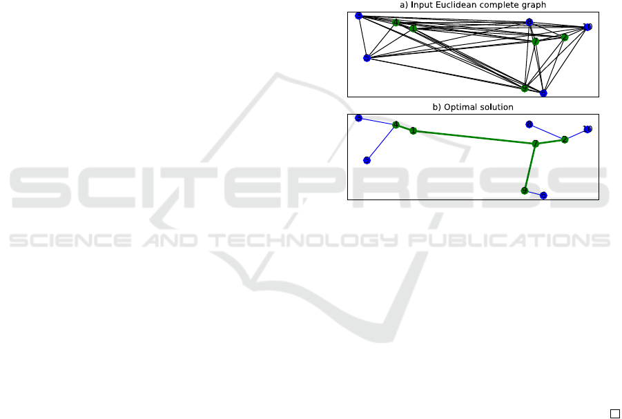
connectivity cost. In Figure 1, we present an exam-

ple of an input complete graph instance composed of

n = 10 nodes and the optimal solution obtained for a

value of p = 5. Recall that an optimal solution to the

problem is also a feasible solution.

As it can be observed from Figure 1, the ﬁve green

nodes and the edges connecting them are part of the

backbone network and form a spanning tree, i.e., an

acyclic connected graph with p − 1 = 4 edges. Simi-

larly, the remaining n − p = 10 − 5 = 5 nodes, which

in this case are also ﬁve, are colored blue and con-

nected to the leaf nodes of the spanning tree formed

with the green nodes. A leaf node of the spanning

tree is a node with a degree equal to one, i.e., a node

having only one neighbor.

Hereafter, we refer and denote by pMST to this

sensor network problem.

Figure 1: Example of a Euclidean input complete graph in-

stance composed of n = 10 nodes and its optimal solution.

Observation 1. For any value of p ∈ {1, . . . , n}, a

feasible solution for pMST corresponds to a spanning

tree composed of n nodes.

Proof. For a particular value of p, the acyclic back-

bone to be obtained will contain p − 1 edges. Since

there are n − p remaining nodes and each one of them

must be connected to a unique leaf node of the re-

sulting backbone structure, then there are n − p addi-

tional edges. Consequently, the total number of edges

is (n − p) + (p −1) = n − 1.

Observation 2 . When p = 1, pMST reduces to ﬁnd

a star graph and its optimal solution can be obtained

in at most O(n) steps.

Observation 3. When p = n, pMST reduces to the

classical minimum spanning tree problem which can

be solved in polynomial time in at most O(m log m)

where m denotes the number of edges of the input

graph (Kruskal, 1956).

Proposition 4. For any value of p ∈ {1, . . . , n} and

n ≥ 3, there are





p−2

≤ n

n−2

labelled spanning

trees in the feasible set of pMST .

On a Wireless Sensor Network Problem with Spanning Tree Backbone

Proof. First, notice that there are





combinations of

nodes to form a spanning tree backbone using p out

of n nodes. Recall that Cayley’s formula ensures that

for each complete graph composed of p nodes, there

are p

p−2

labelled spanning trees (Aigner and Ziegler,

1998). To show that





p−2

≤ n

n−2

, we equivalently

prove that for any value of p ∈ {1, . . . , n −1} and n ≥

3, the following inequality holds





p−2

≤



p + 1



(p +1)

p−1

Notice that this inequality can be equivalently written

(n − p)!p!

p−2

≤

(n − (p + 1))!(p + 1)!

(p +1)

p−1

which can be reduced to

(p +1)p

p−2

≤ (n − p)(p + 1)

p−1

and

(n − p)



p + 1



p−2

≥ 1

The latter is always valid since p ≤ n − 1 and n ≥

Corollary 5. The solution cost of the minimum span-

ning tree of G is a lower bound for the minimum so-

lution cost of pMST .

Proof. This is a consequence of Proposition 4 which

ensures that the number of backbone solution trees to

be formed with p out of n nodes is less than or equal

to the number of solution trees that can be obtained

with n nodes.

2.2 MILP Models

In order to write the ﬁrst MIP model, we deﬁne the

following binary variables

(

1 if node i ∈ V is part of the backbone tree.

0 otherwise.











1 if node i ∈ V is part of the backbone tree

and a leaf node simultaneously.

0 otherwise.

i j











1 if connection link (i, j) ∈ V ×V, (i 6= j)

is part of the backbone tree.

0 otherwise.

and

i j

(

1 if node i ∈ V is connected to leaf node j ∈ V .

0 otherwise.

Notice that even though this last variable x is deﬁned

as a binary one, it can be relaxed within the interval

[0;1] as it always takes values in {0, 1}. This is im-

plied by the constraints (2) in (M

). Consequently, a

ﬁrst MIP model can be written as

) : min

{u,v,x,y,z}

∑

i, j∈V

(i6= j)

i j

+ y

i j

) (1)

s.t.:

∑

j∈V

(i6= j)

i j

+ v

= 1, ∀i ∈ V (2)

i j

≤ z

, ∀i, j ∈ V, (i 6= j) (3)

≤ v

, ∀ j ∈ V (4)

∑

j∈V

= p (5)

∑

i, j∈V

(i6= j)

i j

= p −1 (6)

≤ pv

, ∀ j ∈ V (7)

≥ v

, ∀ j ∈ V (8)

∑

i∈V

(i6= j)

i j

≤ v

, ∀ j ∈ V (9)

− u

− py

i j

− (p − 2)y

≥ 1 − p,

∀i, j ∈ V, (i 6= j) (10)

∑

i∈V

(i6= j)

i j

∑

i∈V

(i6= j)

≤ (p − 1)v

− (p − 2)z

∀ j ∈ V (11)

x ∈ [0, ∞)

, u ∈ [0, ∞)

(12)

y ∈ {0, 1}

, z ∈ {0, 1}

, v ∈ {0, 1}

(13)

In (M

), each entry of the input symmetric matrix

C = (C

i j

), for all i, j ∈ V × V, (i 6= j), represents the

connection cost of nodes i and j. Thus, the objec-

tive function (1) minimizes the total connectivity cost.

Constraints (2) ensure that each node i ∈ V should be

connected to a node of the backbone tree or other-

wise, it should belong to the backbone tree. Similarly,

the constraints (3) ensure that each node i ∈ V should

be connected to node j ∈ V if and only if i is not a

leaf and j is a leaf node of the backbone. The con-

straints (4) ensure that each node j ∈ V can be a leaf

node if it is part of the backbone. Notice that these

constraints are required since a node being part of the

backbone is not always a leaf node. Constraint (5)

ensures that the total number of nodes being part of

the backbone equals p. Subsequently, constraints (6)-

(10) ensure that p out of n nodes of V form a spanning

tree. Notice that these constraints act simultaneously

in order to avoid cycles in the output solution of the

problem. For this purpose an auxiliary nonnegative

variable u

is deﬁned and used for each node i ∈ V .

WINSYS 2021 - 18th International Conference on Wireless Networks and Mobile Systems

For a deeper comprehension of how these constraints

work, we refer the reader to (Desrochers and Laporte,

1991; Adasme et al., 2018; Adasme, 2018). Next, the

constraints (11) ensure that if a particular node j ∈ V

is part of the backbone and if it is chosen to act as

a leaf node, then the degree of j should be equal to

one. Notice that the degree constraint is imposed only

for the nodes of the backbone structure. Obviously,

any leaf node can be connected to several dominated

nodes. Finally, constraints (12) and (13) are domain

constraints for the decision variables.

In order to state a single ﬂow-based formulation

for pMST , we consider the extended set of nodes V ∪

{r} where node r acts as an artiﬁcial root node which

is assumed to be connected to every other node in V .

The underlying idea is to construct an arborescence

rooted at r while sending p units of ﬂow from r with

exactly one arc leaving r. We use the same variables

v, x, y, z as deﬁned for model (M

) and introduce the

nonnegative ﬂow variables f ∈ [0, ∞)

(n+1)

where f

i j

denotes the amount of ﬂow on arc (i, j) ∈ V ∪ {r} ×

V ∪ {r}, (i 6= j). Notice that now the dimensions of

variable v and y are v ∈ {0, 1}

n+1

and y ∈ {0, 1}

(n+1)

respectively. Consequently, a ﬂow-based model can

be written as

) : min

{ f ,v,x,y,z}

∑

i, j∈V

(i6= j)

i j

+ y

i j

)

∑

j∈V

(i6= j)

i j

+ v

= 1, ∀i ∈ V

i j

≤ z

, ∀i, j ∈ V, (i 6= j)

≤ v

, ∀ j ∈ V

∑

j∈V

= p

∑

i, j∈V

(i6= j)

i j

= p −1 (14)

∑

j∈V

r j

= p (15)

∑

j∈V

r j

= 1 (16)

∑

i∈V ∪{r}

(i6= j)

i j

−

∑

i∈V ∪{r}

(i6= j)

= v

, ∀ j ∈ V (17)

i j

≤ py

i j

, ∀i, j ∈ V ∪ {r}, (i 6= j) (18)

= 1 (19)

∑

i∈V

(i6= j)

i j

∑

i∈V

(i6= j)

≤ (p − 1)v

− (p − 2)z

∀ j ∈ V

x ∈ [0, ∞)

, y ∈ {0, 1}

(n+1)

(20)

z ∈ {0, 1}

, v ∈ {0, 1}

n+1

(21)

f ∈ [0, ∞)

(n+1)

(22)

In (M

), constraint (15) ensures that the amount of

ﬂow going from node r to every other node in V

equals p. Similarly, constraint (16) guarantees that

the total ﬂow must be moved through a unique arc

going from r to a unique node j ∈ V . Notice that

the constraints (14), (17) and (18) ensure that the de-

cision variables y = (y

i j

), ∀i, j ∈ V form a spanning

tree backbone using p out of n nodes (Adasme, 2018;

Adasme, 2019). Next, constraint (19) ensures that the

artiﬁcial node r is active. Finally, constraints (20)-

(22) are the domain constraints for the decision vari-

ables.

3 LOCAL SEARCH HEURISTIC

In this section, we present the local search method.

The algorithm is simple and mainly consists of in-

terchanging node elements randomly between subsets

and V

where V

∪ V

= V . The ﬁrst subset con-

tains p nodes whereas the second one contains n − p

nodes. The pseudo-code of the method is depicted in

Algorithm 3.1. As it can be observed, in step one of

Algorithm 3.1, both subsets V

and V

are randomly

generated. Then, with the p nodes of V

, the algo-

rithm constructs p star graphs and for each one, it as-

signs each of the n − p nodes to its nearest leaf node.

Notice that the way in which we construct each span-

ning tree is a key ingredient of our proposed heuristic.

We notice that it is highly probable to obtain spanning

trees in the form of star graphs as we test instances for

values of p << n so far. Next, in step two we enter

into a while loop in which a variable number of swap

moves indK is performed between subsets V

and V

If a better solution is obtained, we save this new so-

lution as the best found so far and reset indK = 1 in

order to further exploit the neighborhood of the in-

cumbent solution. We also save and reset the current

CPU time in order to allow another maxTime units of

time to run the algorithm. Finally, the current num-

ber of iterations is also saved. Otherwise, if no better

solution is obtained, the algorithm restores subsets V

and V

with their previous best subsets of nodes and

increases by one unit the variable indK. In case the

indK variable reaches the maximum value indKMax,

then we also set indK = 1 in order to allow the al-

gorithm to explore from local to wider zones of the

feasible space again.

On a Wireless Sensor Network Problem with Spanning Tree Backbone

Algorithm 3.1: Random local search algorithm for the

pMST problem.

Data: An input complete graph instance

composed of n nodes, an input value of

p < n.

Result: A feasible solution and its objective

function value.

Step 1;

- Generate an initial random p−tuple of vertices.

Let V

denote this set of vertices and V

its

complement.

- Generate p star graphs with the nodes of V

. For

each generated star graph assign each node in V

to its nearest leaf node in V

- Compute the objective function value of each star

graph solution and save the initial and best

feasible solutions obtained.

- V

1OP

= V

, V

2OP

= V

- indK = 1, C puTime = 0.

Step 2;

while (CpuTime ≤ maxTime) do

- iter = iter + 1

for i = 1 to indK do

- Interchange randomly an element of V

with an element of V

- Generate p star graphs with the nodes of V

For each generated star graph assign each

node in V

to its nearest leaf node in V

- Compute the objective function value of each

star graph solution.

if (A better solution is obtained) then

- Save the new solution and set

1OP

= V

, V

2OP

= V

- iterOp = iter, indK = 1,

Optime = Optime +CpuTime,

CpuTime = 0.

else

- V

= V

1OP

, V

= V

2OP

- indK = indK + 1.

if (indK = indKMax) then

- indK = 1.

- Return best solution obtained and its objective

function value.

4 NUMERICAL RESULTS

In this section, we present preliminary numerical re-

sults obtained with the proposed models and with

the Algorithm 3.1. For this purpose, we implement

a Python program using Gurobi 9.1.1 (Achterberg,

2021) in order to solve both MIP models and their

linear programming (LP) relaxations. The numeri-

cal experiments have been carried out on an Intel(R)

64 bits core (TM) with 3 GHz and 8G of RAM un-

der Windows 10. Gurobi solver is used with default

options. We generate ﬁve complete graph instances

with dimensions of n = {40, 80, 120, 150, 200} nodes

using Euclidean and random uniform distance costs.

The random distance costs are drawn from the inter-

val (0;1). All the instances are solved for values of

p = {5, 10} so far. Notice that the number of nodes

of a backbone sensor network is usually smaller than

the number of terminal nodes. In Algorithm 3.1, we

arbitrarily set maxTime = 20s and indKMax = p.

In Table 1, we present preliminary numerical re-

sults obtained with the MIP models. More precisely,

in columns 1-3 we present the instance number, the

value of p, and the number of nodes of graph G, re-

spectively. Next, in columns 4-9 and 10-15 we report

for each model, the best objective function value ob-

tained, the number of branch and bound nodes, CPU

time in seconds required to solve the MIP model, the

objective function value obtained for the LP relax-

ation, its CPU time in seconds and gap values, respec-

tively. The gap values are computed by



Best−LP

Best



∗

100%.

From Table 1, we observe a similar performance

for both models in terms of quality objective function

values and CPU times obtained. Notice that we have

limited the maximum CPU time of the Gurobi solver

to 2 hours. Consequently, when the objective func-

tion value reported is obtained in less than 2 hours,

it means we have found the optimal solution. Other-

wise, we report the best objective function value ob-

tained without proven optimality. Next, we see that

) allows to obtain slightly lower objective func-

tion values than (M

). This observation is also valid

for the CPU time required to solve the MIP models.

Regarding the number of branch and bound nodes,

we observe values of similar orders of magnitude. We

also see that the objective values obtained with the LP

relaxation of (M

) are higher than those obtained with

). This is also conﬁrmed by looking at the gap

values as they are tighter for (M

). In general, we ob-

serve similar trends for the instances using Euclidean

and random distance costs. Finally, we observe that

the objective function values obtained for p = 5 are

higher than those obtained for p = 10. Notice that

this is a consequence of Proposition 4 which states

that the number of solution spanning trees increases

with p.

In Table 2, we present numerical results obtained

with Algorithm 3.1 for the same set of instances in

Table 1. Columns 1-3 are the same as in Table 1.

For the sake of comparison, in columns 4 and 5,

we repeat columns 4 and 6 from Table 1. Next, in

columns 6-10, we report the initial and best objec-

tive function values obtained with Algorithm 3.1, its

CPU time in seconds, the number of iterations re-

quired to get the best solution, and the gaps obtained

when compared to the best objective values of col-

WINSYS 2021 - 18th International Conference on Wireless Networks and Mobile Systems

Table 1: Numerical results obtained with models (M

) and (M

) for complete graph instances with Euclidean and random

distance costs.

# p n

: (MTZ-based model) M

: (Single-ﬂow based model)

Best B&Bn CPU(s) LP CPU(s) Gap % Best B&Bn CPU(s) LP CPU(s) Gap %

Complete graph instances with Euclidean distance cost.

40 7.54 1403 9.61 6.65 0.05 11.77 7.54 2345 31.04 6.59 0.04 12.5

2 80 16.33 9539 547.35 15.14 0.64 7.26 16.33 25747 1593.37 15.09 0.5 7.59

3 120 23.44 1399 466.54 22.47 2.43 4.14 23.44 3044 885.84 22.3 1.49 4.86

4 150 29.6 17387 3844.75 28.52 5.1 3.61 29.6 5337 7200 28.32 2.17 4.29

5 200 37.56 2319 7200 36.4 16.25 3.08 37.49 1272 7200 36.21 6.83 3.4

40 6.12 292462 1295.14 4.33 0.03 29.2 6.12 469415 5421.03 4.2 0.02 31.31

2 80 11.66 58762 7200 8.58 0.47 26.38 11.61 16571 7200 8.55 0.23 26.37

3 120 17.15 14811 7200 13.86 2.49 19.18 17.32 5227 7200 13.75 0.99 20.6

4 150 20.96 10148 7200 18.08 5.46 13.71 22.01 1021 7200 17.98 3.89 18.3

5 200 26.64 1625 7200 23.56 16.95 11.54 26.68 779 7200 23.47 7.56 12.02

Complete graph instances with random distance cost.

40 9.12 173 5.41 7.82 0.07 14.28 9.12 1189 37.81 7.81 0.06 14.37

2 80 17.72 7563 759.38 15.12 0.75 14.67 17.72 12499 1765.01 15.1 1.02 14.77

3 120 28.56 17609 7200 24.79 2.07 13.19 29.2 2556 7200 24.78 2.36 15.14

4 150 36.65 5311 7200 30.97 4.3 15.5 36.74 832 7200 30.96 4.44 15.72

5 200 49.03 884 7200 41.45 9.52 15.46 49.52 132 7200 41.42 9.89 16.36

40 6.21 1558 16.5 4.53 0.03 27.08 6.21 5363 79.91 4.44 0.02 28.59

2 80 11.82 36880 7200 9.25 0.63 21.74 11.82 14743 7200 9.22 0.71 21.98

3 120 18.96 4376 7200 15.53 2.06 18.09 18.87 1936 7200 15.5 1.91 17.82

4 150 24.41 2528 7200 19.32 3.89 20.84 27.6 992 7200 19.3 3.31 30.06

5 200 32.27 1120 7200 25.69 8.84 20.4 37.0 61 7200 25.65 7.99 30.66

Table 2: Numerical results obtained with Algorithm 3.1 for complete graph instances with Euclidean and random distance

costs.

# p n

: (MTZ-based model) Algorithm 3.1

Best CPU(s) Ini Best CPU(s) Iter Gap %

Complete graph instances with Euclidean distance cost.

40 7.54 9.61 15.51 7.54 4.02 4046 0

2 80 16.33 547.35 20.43 16.33 8.27 3912 0

3 120 23.44 466.54 35.67 23.44 8.87 2761 0

4 150 29.6 3844.75 47.89 29.66 10.05 2521 0.22

5 200 37.56 7200 62.96 37.51 27.52 5162 -0.12

40 6.12 1295.14 12.15 6.67 5.64 2794 9.05

2 80 11.66 7200 16.78 11.72 30.41 6715 0.54

3 120 17.15 7200 23.6 17.15 75.74 10579 0

4 150 20.96 7200 28.5 21.34 91.0 10034 1.84

5 200 26.64 7200 39.15 26.79 98.46 8024 0.57

Complete graph instances with random distance cost.

40 9.12 5.41 11.88 9.18 1.23 1167 0.65

2 80 17.72 759.38 24.9 17.87 16.43 7844 0.85

3 120 28.56 7200 36.34 29.0 10.32 3335 1.56

4 150 36.65 7200 44.12 36.42 16.79 4247 -0.62

5 200 49.03 7200 54.78 48.19 28.74 5443 -1.69

40 6.21 16.5 10.07 6.77 2.44 1143 9.14

2 80 11.82 7200 20.27 12.13 47.7 10368 2.68

3 120 18.96 7200 27.75 19.55 23.05 3240 3.11

4 150 24.41 7200 32.8 24.04 153.26 17125 -1.5

5 200 32.27 7200 41.48 32.46 104.45 8316 0.6

umn 4 of Table 2. These gap values are computed by

Best(M

)−Best(Heuristic)

Best(M

)

∗ 100% where Best(M

) de-

notes the best objective value reported in column 4 of

Table 2 and Best(Heuristic) the best objective value

reported in column 7 of Table 2, respectively.

From Table 2, we observe that the initial objec-

tive values obtained with Algorithm 3.1 are signiﬁ-

cantly larger than the best ones. This fact evidences

the effectiveness of Algorithm 3.1. Then, we see that

the best objective values obtained are near-optimal for

most of the instances. This can be veriﬁed by looking

at the gap column as well. Notice that the instances

with negative gaps indicate that better solutions are

obtained with Algorithm 3.1 compared to the solu-

tions obtained with the MIP models. The CPU time

values required by the algorithm are remarkably lower

than those required by the MIP models. Notice that

most of the instances are solved by the algorithm in

On a Wireless Sensor Network Problem with Spanning Tree Backbone

less than 100 seconds in contrast to the two hours re-

quired by the MIP solver.

5 CONCLUSIONS

In this paper, we represent a wireless sensor network

by means of a complete graph G = (V, E) with a set

of nodes V and a set of edges E. Then, we consid-

ered the problem of ﬁnding a minimum spanning tree

backbone formed with a subset of nodes P ⊆V where

the remaining nodes belonging to subset V \ P must

be connected to the leaf nodes of subset P at mini-

mum total connectivity cost. The problem is mainly

motivated as it can be used for comparison purposes

when developing future network protocols for these

types of networks. We proposed two mixed-integer

programming formulations for the problem and a lo-

cal search heuristic that allows obtaining feasible so-

lutions in less computational effort. So far, we tested

complete graph instances with random uniform and

Euclidean distance costs. Our preliminary numeri-

cal results showed that one of the proposed models

outperforms the other one in terms of solution qual-

ity and CPU times obtained with the Gurobi solver.

Finally, the proposed heuristic allows one to obtain

near-optimal solutions in signiﬁcantly less CPU time

and better solutions for some of the instances when

compared to the MIP models.

As future research, we plan to propose new for-

mulations and solving methods for the problem. In

particular, novel exact and suboptimal approximation

methods should be investigated in order to compare

with the proposed heuristic.

ACKNOWLEDGEMENTS

The authors acknowledge the ﬁnancial support from

Projects: FONDECYT No. 11180107 and FONDE-

CYT No. 3190147.

REFERENCES

Achterberg, T. (2021). Gurobi solver,

https://www.gurobi.com/.

Adasme, P. (2018). p-median based formulations with

backbone facility locations. Applied Soft Computing,

67:261–275.

Adasme, P. (2019). Optimal sub-tree scheduling for wire-

less sensor networks with partial coverage. Computer

Standards & Interfaces, 61:20–35.

Adasme, P., Andrade, R., Leung, J., and Lisser, A. (2018).

Improved solution strategies for dominating trees. Ex-

pert Systems with Applications, 100:30–40.

Adasme, P., Andrade, R., and Lisser, A. (2017). Minimum

cost dominating tree sensor networks under proba-

bilistic constraints. Computer Networks, 112:208–

222.

Aigner, M. and Ziegler, G. (1998). Proofs from THE BOOK.

Springer-Verlag.

BenSaleh, M. S., Saida, R., Kacem, Y. H., and Abid, M.

(2020). Wireless sensor network design methodolo-

gies: A survey. Journal of sensors, 2020:1–13.

Chowdhury, M. Z., Hasan, M. K., Shahjalal, M., Hossan,

M. T., and Jang, Y. M. (2020). Optical wireless hy-

brid networks: Trends, opportunities, challenges, and

research directions. IEEE Communications Surveys &

Tutorials, 22(2):930–966.

Desrochers, M. and Laporte, G. (1991). Improvements

and extensions to the miller-tucker-zemlin subtour

elimination constraints. Operations Research Letters,

10:27–36.

Hansen, P. and Mladenovic, N. (2001). Variable neighbor-

hood search: Principles and applications. European

Journal of Operational Research, 130:449–467.

Huang, J., Liu, Y., Wang, C. X., Sun, J., and Xiao, H.

(2019). 5g millimeter wave channel sounders, mea-

surements, and models: Recent developments and fu-

ture challenges. IEEE Communications Magazine,

57(1):138–145.

Jiang, W., Han, B., Habibi, M. A., and Schotten, H. D.

(2021). The road towards 6g: A comprehensive sur-

vey. IEEE Open Journal of the Communications So-

ciety, 2:334–366.

Kruskal, J. B. (1956). On the shortest spanning subtree of

a graph and the traveling salesman problem. Proceed-

ings of the American Mathematical Society, 7:48.

Martin, I. R., Gonzalez, J. J. S., and Yaman, H. (2014).

A branch-and-cut algorithm for the hub location and

routing problem. Computers & Operations Research,

50:161–174.

Mladenovic, N. and Hansen, P. (1997). Variable neighbor-

hood search. Computers and Operations Research,

24:1097–1100.

Yaman, H. and Elloumi, S. (2012). Star p-hub center prob-

lem and star p-hub median problem with bounded

path lengths. Computers & Operations Research,

39(11):2725–2732.

WINSYS 2021 - 18th International Conference on Wireless Networks and Mobile Systems