Path Planning in Unstructured Urban Environments for
Self-driving Cars
Anderson Mozart, Gabriel Moraes, Rânik Guidolini, Vinicius B. Cardoso, Thiago Oliveira-Santos,
Alberto F. De Souza
*
and Claudine Badue
Departamento de Informática, Universidade Federal do Espírito Santo, Vitória, Brazil
Keywords: Path Planning, Unstructured Urban Environments, Self-driving Cars, A* Algorithm.
Abstract: We present a path planner for unstructured urban environments (PPUE) for self-driving cars. PPUE receives
initial and goal poses as input, as well as maps of the environment. It employs a hybrid A* algorithm with
two heuristics for generating paths, which are smoothed using Conjugate Gradient optimization. Different
from previous works, PPUE uses: (i) an obstacle distance grid-map, instead of an occupancy grid-map, for
representing the environment; and (ii) an accurate but simple collision model of the car. We have examined
PPUE’s performance experimentally in simulated and real world scenarios. Our results show that PPUE
computes smooth and safe paths, which follow the kinematic constraints of the vehicle, fast enough for
suitable real world operation.
*
Senior Member, IEEE
1 INTRODUCTION
The path planning task of self-driving cars can be
formulated as the problem of finding a sequence of
poses, 𝑃={𝑝

,𝑝

,…,𝑝

,…,𝑝
||
}, from the current
car pose, 𝑝

, to a desired pose, 𝑝
||
, where each
pose is a position in the world, defined as a 2-D
coordinate pair, the self-driving car’s orientation at
this position, and the direction of movement
(forward or reverse), i.e., 𝑝

=(𝑥

,𝑦

,𝜃

,𝑟

) .
Depending on the operating scenario, path planning
can be more or less complex. Urban self-driving cars
typically have two main operating scenarios: road
driving and parking. In road driving, path planning
is typically simpler thanks to the road-network
structure. To improve safety, roads have vertical and
horizontal signalizations that simplify driving, and,
therefore, path planning on them. Path planning on
parking lots and other non-structured areas cannot
benefit much of vertical and horizontal signalization,
which makes path planning in such scenarios more
complex.
We have developed a self-driving car, named
Intelligent Autonomous Robotic Automobile (IARA,
Figure 1), whose autonomy system follows the
typical architecture of self-driving cars (Badue et al.,
2020). Our self-driving car is based on a Ford
Escape Hybrid tailored with a variety of sensors and
processing units. Its autonomy system is composed
of many modules, which include a localizer
(Veronese et al., 2016), a mapper (Mutz et al.,
2016), a moving obstacle tracker (Sarcinelli et al.,
2019), a traffic signalization detector (Possatti et al.,
2019; Torres et al., 2019), a route planner, a path
planner for structured urban areas, a behavior
selector, a motion planner (Cardoso et al., 2017), an
obstacle avoider (Guidolini et al., 2016), and a
controller (Guidolini et al., 2017), among other
modules.
In this paper, we propose a path planner for
unstructured urban environments (PPUE) for our or
any other self-driving car. The proposed path
planner for unstructured urban environments (for
now on, path planner for short) is similar to that
presented by Dolgov et al. (2010) – one of the most
preeminent path planners in the literature based on
the A* algorithm – but improve on it in several
aspects. The contributions of this paper are these
improvements, which can be summarized as: (i) the
use of an obstacle distance grid-map instead of an
occupancy grid-map (Thrun, Burgard & Fox, 2006)
to represent the environment; and (ii) a more
accurate but simple collision model of the car, which
290
Mozart, A., Moraes, G., Guidolini, R., Cardoso, V., Oliveira-Santos, T., F. De Souza, A. and Badue, C.
Path Planning in Unstructured Urban Environments for Self-driving Cars.
DOI: 10.5220/0010559602900300
In Proceedings of the 18th International Conference on Informatics in Control, Automation and Robotics (ICINCO 2021), pages 290-300
ISBN: 978-989-758-522-7
Copyright
c
 2021 by SCITEPRESS – Science and Technology Publications, Lda. All rights reserved

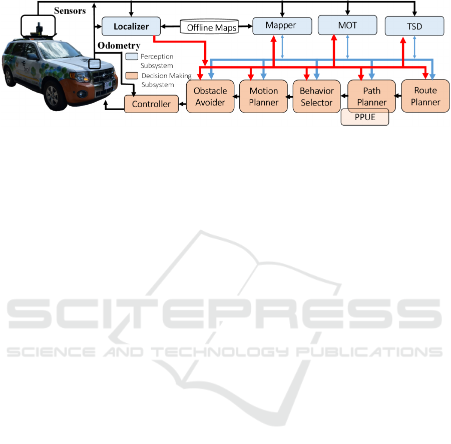
Figure 1: Intelligent Autonomous Robotic Automobile (IARA) and its autonomy software system. In light blue, perception
modules. In orange, decision making modules. TSD denotes Traffic Signalization Detection and MOT, Moving Objects
Tracking. Red arrows show the State of the car, produced by its Localizer module and shared with most modules; blue
arrows show the car’s internal representation of the environment, jointly produced by several perception modules and
shared with most decision making modules. See details in Badue et al. (2020).
simplifies the implementation of the path planner
algorithm. To evaluate the performance of the
proposed path planner, we employed our self-driving
car simulator and different scenarios where the car
had to make different maneuvers to achieve the goal.
We measured the hybrid A* search running time, the
full running time (which includes path smoothing
step), the number of nodes expanded by the hybrid
A* search, and the length of the final smoothed path.
To assess the benefits of the use of the obstacle
distance grid-map and the collision model of the car,
we also measured the running time to create the map
and to query it for the distance from the car to the
nearest obstacle. Finally, we conducted real-world
experiments using our self-driving car in a parking
lot to examine the real world performance of the
solution. Experimental results have shown that our
planner allows our self-driving car to find a proper
path in an unstructured environment in reasonable
time, with running times from 0.42 s to 0.61 s for a
path of about 70 m.
2 RELATED WORKS
Several techniques have been proposed in the
literature for implementing path planners for non-
structured urban environments. Relevant path
planner implementations include graph search based
planners (Dolgov et al., 2010; Chu et al., 2015;
Yoon et al., 2015; Urmson et al., 2008; Wang, 2019)
sample based planners (Ghosh et al., 2019), and
deep neural network based planners (Kicki, Gawron
& Skrzypczyński, 2020; Moraes et al., 2020).
Among those based on graph search, Dolgov et al.
(2010) presented a path planner based on the hybrid
A* algorithm for the autonomous car Junior, that
finished second in the 2007 DARPA Urban
Challenge (Montemerlo et al., 2018). Our path
planner is similar to that of Dolgov et al. (2010), but
refines it in two main aspects: the use of an obstacle
distance grid-map (instead of an occupancy grid-
map) and of a more precise collision model of the
car, which allowed computing the distance from the
car to the nearest obstacle accurately and quickly.
Other authors propose other variants of the A*
algorithm for path planning. Urmson et al. (2008)
proposed the anytime D* to compute a path for the
self-driving car Boss (Carnegie Mellon University’s
car that claimed first place in the 2007 DARPA
Urban Challenge). Both anytime D* and hybrid-state
A* algorithms merge two heuristics – one non-
holonomic, which disregards obstacles, and the other
holonomic, which considers obstacles – and were
used for path planning in an unstructured
environment (parking lot). Chu et al. (2015)
proposed a variation of A* to build a path that
considers car’s kinematic constraints, which ignores
the resolution of grid cells and creates a smooth
path. Yoon et al. (2015) proposed a variation of A*
to compute a path that accounts for kinematic
constraints of the autonomous vehicle Kaist. None
of these works use obstacle-distance maps.
Wang (2019) proposes a variant of the Hybrid
A* (i-AGT) that conducts selective expansion for a
node, where only the control actions with the highest
priority are applied, and a bidirectional A-search
(BAGT), where two trees are constructed
simultaneously from the initial and goal state. The
path planner was tested in a simulation of a car in a
parking lot, and its computation time, complexity of
the tree and path length were measured.
Experimental results indicate that i-AGT and BAGT
are significantly faster than the normal Hybrid A*,
Path Planning in Unstructured Urban Environments for Self-driving Cars
291

but in some cases, the BAGT is prone to fail (Wang,
2019).
Among those based on sampling, Ghosh et al.
(2019) propose a kinematically constrained Bi-RRT
(KB-RRT) algorithm, where the expansion of RRT
is restricted to feasible regions of the state space,
which avoids unnecessary growth of the RRT. In
this approach, two RRTs are created from the initial
and goal state, and are grown until they become
connected, when a solution is found. This solution
does not guarantee an optimal trajectory, however.
Among those techniques based on neural
networks, Kicki, Gawron and Skrzypczyński (2020)
presented a path planner that employs a gradient
based self-supervised learning algorithm to predict
feasible paths. The neural network receives a
representation of the environment, the initial and
desired final robot poses, and generates a path spline
defined as a 5-th degree polynomial. They evaluated
the performance of their path planner in simulation
experiments, in which overtaking maneuvers,
perpendicular parking and oblique parking were
considered. Their experimental results showed that
their path planner can be 14 times faster than other
comparing planners and serve as a generator of the
initial solutions for other complete path planning
algorithms. Moraes et al. (2020) presented an image-
based path planner for self-driving cars, which
receives a front-face camera image and the current
car pose, infers a cubic spline path model, generates
the path in the car coordinate system and transforms
its poses to the world coordinate system. They
examined the performance of their path planner in
real world scenarios. Their experimental results
showed that the path planner is capable to generate
paths on straight and curved sections of the lane, but
might fail on forks in the road. Path planner based
on neural networks does not guarantee optimality
nor completeness, however.
3 A PATH PLANNER FOR
UNSTRUCTURED
ENVIRONMENTS
The hybrid-state A* algorithm of PPUE receives as
input the Initial Pose, 𝑝

, the Final Pose, 𝑝
||
, an
Obstacle Distance Grid-Map ( 𝐎𝐃𝐆𝐌 ), a Goal
Distance Map ( 𝐆𝐃𝐌 ), and a Nonholonomic
Heuristic Cost Map ( 𝐍𝐇𝐂𝐌 ). Each cell of the
𝐎𝐃𝐆𝐌 holds the distance from itself to the nearest
obstacle – the way we compute this map online and
the benefits of using it are described in Section 3.2.
Each cell of 𝐆𝐃𝐌 holds the length (travelled
distance) of a holonomic path from itself to the goal
considering obstacles – see Section 3.4. Finally,
each cell of 𝐍𝐇𝐂𝐌 holds the length of a
nonholonomic path from itself to the goal without
considering obstacles – the cost of computing this
map is high, but we can compute it only once and
offline, as detailed in Section 3.5. The output of the
hybrid-state A* algorithm is an optimal path 𝑃′ =
{𝑝

,𝑝

,…,𝑝

,…,𝑝
||
}, which may not be suitably
smooth for an Ackermann steering robot. Therefore,
we smooth this path producing the path 𝑃 , as
described in Section 3.8. The smoothed path is sent
to the Behavior Selector module for execution (see
Figure 1). Our implementation of the hybrid-state
A* algorithm is presented in Algorithm 1 and
detailed below.
Algorithm 1: Hybrid-State A* Algorithm.
Input: 𝑝

,𝑝
||
,𝐎𝐃𝐆𝐌,𝐆𝐃𝐌,𝐍𝐇𝐂𝐌
Output: 𝑃
1: 𝑛

←(𝑝

,0,0,NULL)
2: 𝐆𝐒𝐌[.]← (Not visited, 0)
3: 𝐹𝐻 ← {𝑛

}
4: 𝐆𝐒𝐌[𝑛

.𝑝] ← (Open, 𝑔
(
𝑛

)
)
5: 𝐰𝐡𝐢𝐥𝐞 𝐹𝐻 ≠ ∅ 𝐝𝐨
6: 𝑛 ← FH.pop() // get node 𝑛 with minimum 𝑛.f from FH
7: if 𝐆𝐒𝐌[𝑛.p].s ≠ Closed then
8: 𝐆𝐒𝐌[𝑛.𝑝].close()
9: if is_goal(𝑛.𝑝,𝑝
||
) then
10: 𝑃′ = get_path(𝑛)
11: return 𝑃′
12: else
13: 𝑁 ← {expand_node(𝑛, 𝐎𝐃𝐆𝐌)}
14: for n′∈𝑁 do
15: 𝑛′. 𝑔 ← 𝑔(𝑛′)
16: 𝑛′. 𝑓 ← 𝑓(𝑛′)
17: 𝑛′. 𝑝𝑎𝑟𝑒𝑛𝑡 ← 𝑛
18: if 𝐆𝐒𝐌[n′. 𝑝].s ≠ Closed and
19: (𝐆𝐒𝐌[n′.𝑝].s = Not visited or
20:
(𝐆𝐒𝐌[n′.𝑝].s = Open and 𝐆𝐒𝐌[𝑛′.𝑝].g > 𝑛′.𝑔)) then
21: 𝐆𝐒𝐌[n′. 𝑝] = (Open, 𝑛′.𝑔)
22: 𝐹𝐻 ← 𝐹𝐻 ∪
{
𝑛

}
23: return {∅} // path not found
3.1 Hybrid A* Search
Different from the standard A*, where the search is
performed in a graph, in the hybrid-state A*
algorithm the search is performed in a Grid State
Map (𝐆𝐒𝐌). Algorithm 1 finds 𝑃′ using the 𝐆𝐒𝐌
and a Fibonacci Heap, 𝐹𝐻, of nodes
. 𝐆𝐒𝐌 is a 4D
grid-map indexed by discretized poses, 𝑝

=
(𝑥

,𝑦

,𝜃

,𝑟

), where each cell holds a state and a
value. The state can be “Not visited”, “Open”, or
“Closed”, while the value is computed by a path-cost
function, 𝑔(.). We use the Fibonacci Heap, 𝐹𝐻, for
efficiently implementing the list of nodes being
handled by the algorithm at each instant of time.
ICINCO 2021 - 18th International Conference on Informatics in Control, Automation and Robotics
292

Each node, 𝑛, holds: a candidate pose of 𝑃′; the cost
𝑓, computed by the cost function 𝑓(.); the cost 𝑔,
computed by the cost function 𝑔(.); and a pointer to
its parent node. In the following, we detail these cost
functions.
The hybrid A* algorithm is guided by the costs
𝑓 and 𝑔 of each node. It tries and finds a path from
𝑝

to 𝑝
||
traversing 𝐆𝐒𝐌 through the cells with the
smallest f and 𝑔, starting with the cell set with 𝑝

.
To examine all possible paths allowed by the
discretization of the space provided by 𝐆𝐒𝐌 is too
expensive; hence, the use of a search algorithm
such as the hybrid A* is a practical alternative.
Starting from an initial node we call 𝑛

, which is
set using 𝑝

(line 1 of Algorithm 1), the algorithm
expands new nodes, 𝑛’ , whose poses obey the
robot’s nonholonomic restrictions and that do not
collide with obstacles. The costs 𝑓 and 𝑔 of 𝑛’ are
computed by the functions 𝑓(𝑛’) and 𝑔(𝑛’), which
are given by
𝑓
(
𝑛′
)
=𝑝𝑒𝑛𝑎𝑙𝑡𝑖𝑒𝑠
(
𝑛

)
+𝑔
(
𝑛′
)
+ℎ
(
𝑛′
)
(1)
and
𝑔
(
𝑛′
)
=𝑔
(
𝑛
)
+
|
𝑛.𝑝 − 𝑛

.𝑝
|
,
(2)
where
ℎ
(
𝑛′
)
=max (𝐆𝐃𝐌
[
𝑛

.𝑝
]
,𝐍𝐇𝐂𝐌𝑝
|

|
−𝑛′.𝑝).(3)
So, as shown in (1), 𝑓
(
𝑛′
)
is the sum of the costs
associated with 𝑛′. Let’s start by examining the costs
associated with 𝑛′ by the 𝑝𝑒𝑛𝑎𝑙𝑡𝑖𝑒𝑠(𝑛′) term in (1).
𝑝𝑒𝑛𝑎𝑙𝑡𝑖𝑒𝑠(𝑛′) are given by
𝑝𝑒𝑛𝑎𝑙𝑡𝑖𝑒𝑠
(
𝑛

)
=

𝐎𝐃𝐆𝐌
[


.
]
+
𝑤

×
|
𝑛.𝑝 − 𝑛

.𝑝
|
×𝑛

.𝑝.𝑟+
𝑤

× [𝑛

.𝑝.𝑟≠𝑛.𝑝.𝑟],
(4)
where 𝑤

and 𝑤

are weights.
In (4) and throughout the text, we use the
notation 𝑥.𝑦 to refer to the element 𝑦 of 𝑥 (𝑛

.𝑝 is
the pose element of 𝑛′ ). So, by its first term,
𝑝𝑒𝑛𝑎𝑙𝑡𝑖𝑒𝑠
(
𝑛′
)
grows with the inverse of the
distance between the pose of the node 𝑛’ and the
nearest obstacle. By the second term, 𝑝𝑒𝑛𝑎𝑙𝑡𝑖𝑒𝑠
(
𝑛′
)
increases with 𝑤

times the Euclidean distance
between the poses of the nodes 𝑛 and 𝑛’ if the
direction of movement from 𝑛 to 𝑛’ is reverse (i.e.,
𝑛

.𝑝.𝑟=1 ). Finally, by the third term,
𝑝𝑒𝑛𝑎𝑙𝑡𝑖𝑒𝑠
(
𝑛′
)
increases with 𝑤

in case of a change
in the direction of movement (i.e., 𝑛

.𝑝.𝑟≠𝑛.𝑝.𝑟).
The weights 𝑤

and 𝑤

are parameters of the
algorithm.
The next term of (1) is 𝑔
(
𝑛′
)
itself, which is
given by (2). As shown in (2), 𝑔
(
𝑛′
)
is equal to 𝑔
(
𝑛
)
plus the Euclidean distance between the poses of the
nodes 𝑛 and 𝑛′. Finally, the last term of (1) is ℎ
(
𝑛′
)
,
which is given by (3). As shown in (3), ℎ
(
𝑛′
)
is
given by the maximum of two terms: 𝐆𝐃𝐌
[
𝑛′.𝑝
]
and 𝐍𝐇𝐂𝐌𝑝
|

|
−𝑛′.𝑝. The first term represents
the cost of going from 𝑛′.𝑝 to 𝑝
|

|
following a path
that considers obstacles, but not the nonholonomic
restrictions of the car. We detail how we build 𝐆𝐃𝐌
online in Section 3.4. The second term represents the
cost of going from 𝑛′.𝑝 to 𝑝
|

|
following a path that
obeys the nonholonomic restrictions of the car, but
that does not consider obstacles. This second term is
important for increasing the cost of paths that arrive
at the goal with wrong robot orientation. We detail
how we build the 𝐍𝐇𝐂𝐌 offline and how we use it
online to compute this cost in Section 3.5.
Algorithm 1 starts by initializing the initial node,
𝑛

, with the tuple (𝑝

,0,0,NULL), in line 1, the
whole 𝐆𝐒𝐌 with the tuple (Not visited, 0), in line 2,
and 𝐹𝐻 with a list of nodes containing 𝑛

only, in
line 3. After this initialization and before the main
loop, in line 4 the algorithm sets the cell of 𝐆𝐒𝐌
where 𝑝

is mapped to with the tuple (Open, 𝑔
(
𝑛

)
).
This marks this cell as Open and sets the cost of this
cell according to the function 𝑔(.).
The main loop of Algorithm 1 starts by testing if
𝐹𝐻 is empty, in line 5, which will not be the case at
start time due to its initialization in line 3. In line 6,
the algorithm gets the node 𝑛 with minimum cost 𝑓
from 𝐹𝐻. The algorithm proceeds by examining if
the cell indexed by the pose of the node 𝑛 is closed,
in line 7. If it is not closed, in line 8, the algorithm
closes the cell. Then, the algorithm checks, in line 9,
if the current node is near enough to the goal using
the function is_goal(). In this case, it computes the
path using get_path(), which basically goes back in
the sequence of nodes from the current node, 𝑛, up
to initial node, 𝑛

, using the pointer to the parent
node that every node maintains, and returns the path
𝑃′, in line 11. If is_goal() returns false, the algorithm
continues from line 12 onwards.
In line 13, the current node taken from 𝐹𝐻 is
expanded producing a set of nodes we call 𝑁 (the
function expand_node() is described in Section 3.6).
This expansion is the mechanism employed by the
algorithm to search for a solution in a space of
alternatives where it can move forwards, backwards,
left, right, or straight. For the set of possible
expansions, the algorithm, starting in line 14,
examines each one of the expansion alternatives and
computes, for each one of them, represented by 𝑛′,
Path Planning in Unstructured Urban Environments for Self-driving Cars
293

𝑛′.𝑔, 𝑛′.𝑓 and the pointer to the parent of 𝑛′, i.e., 𝑛,
in lines 15 to 17, respectively.
Once 𝑛′ is computed, in lines 18 to 20, the
algorithm examines if its cell of 𝐆𝐒𝐌 is not closed,
in line 18, and not visited, in line 19, or if its cell is
open and the value 𝑔 of the cell is larger than the
value 𝑔 of 𝑛′. If the conditions examined in lines
18 to 20 hold true, the cell of 𝐆𝐒𝐌 pointed by the
pose of 𝑛′ is set as open and the value of the cell of
𝐆𝐒𝐌 is set to the value 𝑔 of the node 𝑛′, in line 21.
Then, this node is added to the Fibonacci heap 𝐹𝐻,
in line 22. After examining all possible expansions
of node 𝑛 in lines 13 to 22, the algorithm goes back
to line 5 and checks if the Fibonacci Heap is
empty. If not, it takes the node with the minimum
value 𝑓 from the heap – many of them might have
been added in line 22 – and continues the process,
trying to find a node that is near enough to the goal
as tested in line 9. If one such node is found, the
path 𝑃′ has been found and it is returned by the
algorithm in line 11. If no path is found after
exploring all possible cells of 𝐆𝐒𝐌, the Fibonacci
Heap will be found empty in line 5; that is, there
will be no more nodes to examine. In this case, the
algorithm will terminate in line 23 returning an
empty path.
3.2 Obstacle Distance Grid-Map
(ODGM)
A contribution of this paper is the use of an 𝐎𝐃𝐆𝐌
instead of an occupancy grid-map (Dolgov et al.,
2010) to represent the obstacles in the environment.
Each cell of 𝐎𝐃𝐆𝐌 keeps its distance to the nearest
obstacle; so, to find out the distance from a position
to the nearest obstacle, we simply query the 𝐎𝐃𝐆𝐌
cell where the position is mapped to.
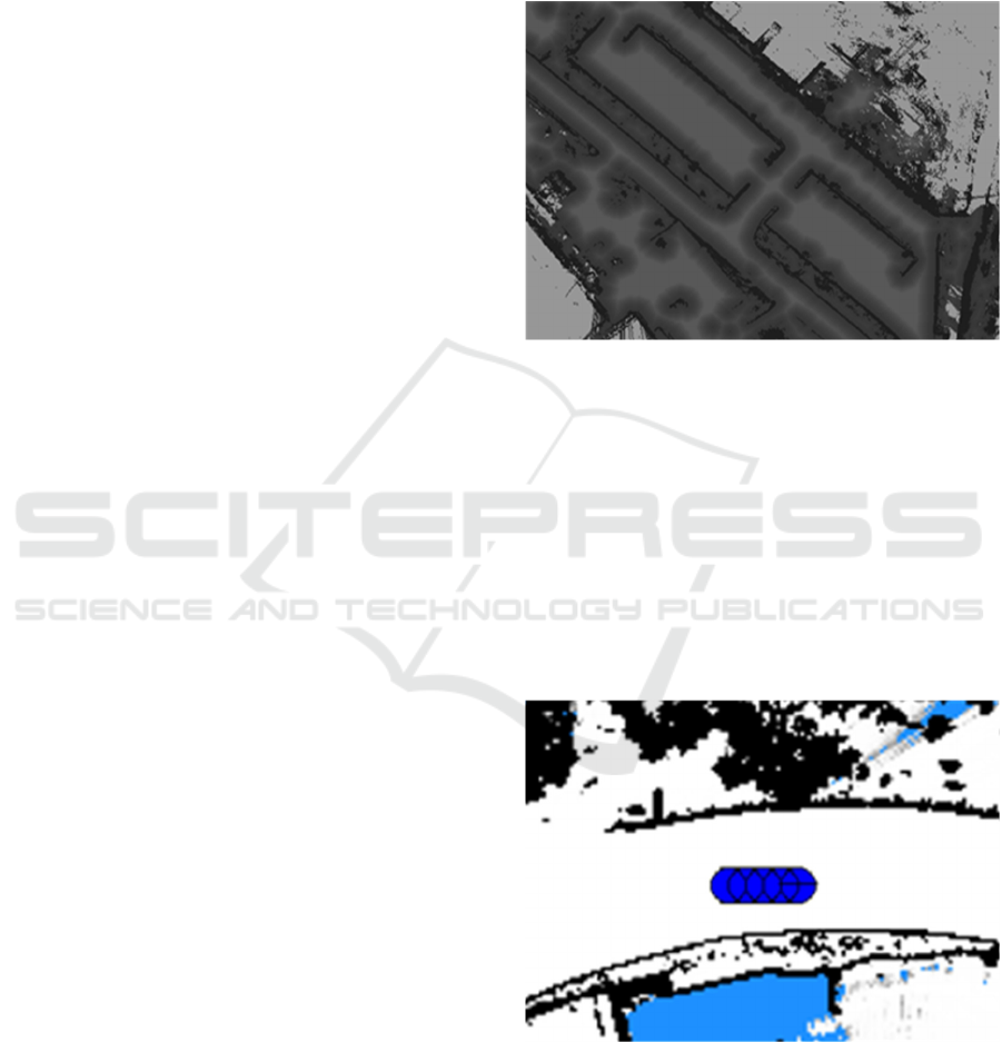
Figure 2 illustrates an 𝐎𝐃𝐆𝐌 of the parking lot
where we conducted real-world experiments using
our self-driving car. In the 𝐎𝐃𝐆𝐌 of Figure 2,
darker cells represent regions closer to obstacles,
while lighter cells indicate areas farther from
obstacles. The uniformly lighter cells in the middle
of the map represent areas whose distances from
obstacles are greater than a threshold and are
represented by a constant value. 𝐎𝐃𝐆𝐌 is computed
online using the current occupancy grid-map of the
same area and dynamic programming.
3.3 Collision Model of the Car
Another contribution of this paper is the use of a
precise, yet simple collision model of the car to
compute the distance from the car to the nearest
obstacle in the context of unstructured path
planning. The collision model of the car is used to:
(i) compute the first term of 𝑝𝑒𝑛𝑎𝑙𝑡𝑖𝑒𝑠
(
𝑛′
)
, in (4)
(see Section 3.1); (ii) verify if expanded nodes, 𝑛’,
collide with obstacles (Section 3.6); and (iii) check
for collisions during path smoothing (Section 3.8).
Figure 2: ODGM. Darker cells represent regions closer to
obtacles, while lighter cells farther from obstacles.
The car is modeled by a set of 5 equally spaced
circles with equal radii, 𝑅. To obtain the distance
from the car to the nearest obstacle, we verify the
obstacle distance held by the 𝐎𝐃𝐆𝐌 cells to where
the centers of the car model circles mapped, and
return the smallest distance. If the returned distance
is smaller than 𝑅, it is considered as collision. Figure
3 shows the collision model of the car (five circles)
with an excerpt from an occupancy grid map in the
background.
Figure 3: Collision model of the car (five circles)
superimposed on a blue rectangle with an excerpt from an
occupancy grid map in the background. The blue rectangle
indicates the current car’s pose. In the occupancy grid map
in the background, white cells represent free regions, grey
cells represent occupied regions and blue cells represent
unknown regions.
ICINCO 2021 - 18th International Conference on Informatics in Control, Automation and Robotics
294

3.4 Goal Distance Map (GDM)
Each cell of 𝐆𝐃𝐌 holds the distance from itself to
the goal, 𝑝
||
. To compute a 𝐆𝐃𝐌, we use the Exact
Euclidean Distance Transform (EEDT), proposed by
Elizondo-Leal, Parra-González, and Ramírez-Torres
(2013) which receives as input a discretized version
of the current 𝐎𝐃𝐆𝐌 and 𝑝
||
. We discretize 𝐎𝐃𝐆𝐌
using a distance threshold (0.5 m) – cells closer to
obstacles than this threshold are set to 1, otherwise,
zero.
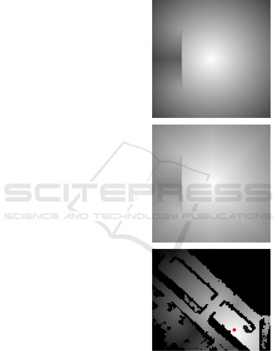
In Figure 4(a), we show an example of 𝐆𝐃𝐌
computed using EEDT, where the goal is the center
of the map and there is only a vertical line as
obstacle. In Figure 4(b), we show the same example,
but using dynamic programming for computing
𝐆𝐃𝐌 . As can be seen in these figures, EEDT
provides a more precise map. 𝐆𝐃𝐌s computed using
dynamic programing have the disadvantage of
making search algorithms prefer paths that follow
the artifacts present in maps produced this way (the
lines in form of star irradiating from the goal in
Figure 4(b)).
In Figure 4(c), we show the 𝐆𝐃𝐌 of a parking
lot used in the experiments. The goal 𝑝
||
is
represented by a small red circle. As can be seen in
the figure, we use a 𝐆𝐃𝐌 with reduced resolution
for closing gaps present in 𝐎𝐃𝐆𝐌 that would
otherwise allow misguided distances to goal in
𝐆𝐃𝐌.
3.5 Nonholonomic Heuristic Cost Map
(NHCM)
Each cell of 𝐍𝐇𝐂𝐌 holds the nonholonomic
distance from 𝑛′.𝑝 to the 𝐍𝐇𝐂𝐌 center, which
represents the goal, 𝑝
|

|
. We access a cell in this map
using the vector 𝑣
(
𝑥,𝑦,𝜃
)
=𝑝
|

|
−𝑛′.𝑝 (see (3));
so, 𝐍𝐇𝐂𝐌 is a tridimensional map indexed by a
discretized version of 𝑣 . We used Reed-Shepp
curves (Reeds & Shepp, 1990) to compute this map.
The cost stored in each cell 𝐍𝐇𝐂𝐌𝑝
|

|
−𝑛′.𝑝 is
equal to the length of the Reed-Shepp curve that
takes the car from a pose 𝑛′.𝑝 to 𝑝
|

|
. The length of
this curve (or path) depends heavily on the
orientation of the current pose, 𝑛′.𝑝, and the Final
Pose, 𝑝
||
. In our implementation, 𝐍𝐇𝐂𝐌 does not
consider obstacles; so, as Dolgov et al. (2010), we
were able to compute it offline and store it as a
lookup table.
(a)
(
b
)
(c)
Figure 4: (a) Example of GDM obtained by EEDT. (b)
Same example of (a) but computed using dynamic
programming. (c) GDM of a parking lot used in
experiments.
Path Planning in Unstructured Urban Environments for Self-driving Cars
295

3.6 Expansion of Nodes
Since we use a nonholonomic robot (a car), the
expansion of a node must follow its kinematic
constraints. The method expand_node() of
Algorithm 1 performs node expansion and receives
the current node, 𝑛 , and 𝐎𝐃𝐆𝐌 as input.
expand_node() computes a set, 𝑁, composed of up
to 6 poses 𝑛′.𝑝 . These poses are computed
simulating the car movement from 𝑛.𝑝 to poses
resulting from moving the car forwards and
backwards for a fixed distance, 𝑑, while steering to
max-left, straight, and to max-right. This results in 6
𝑛′.𝑝 poses. However, if any of these poses results in
a collision in 𝐎𝐃𝐆𝐌, it is not include in the set 𝑁.
3.7 Goal Proximity Verification and
Reed-Shepp Path
The method is_goal() verifies if the current node, 𝑛,
is close enough to the goal and, if it is, the search
terminates. If it is not, is_goal() computes, for every
𝑘(.) nodes examined, where 𝑘(.) is a function that
returns a value that decreases as 𝑛.𝑝 gets closer to
the Final Pose, 𝑝
|

|
, a Reed-Shepp path between 𝑛.𝑝
and 𝑝
|

|
. If the Reed-Shepp-path’s poses have no
collisions and there is no change of direction of
movement in this path, (i) it is appended to the path
computed so far from 𝑛

.𝑝

to 𝑛.𝑝, (ii) 𝑛 receives
the value of the last node of the Reed-Shepp path,
and (iii) is_goal() returns true. Otherwise, is_goal()
returns false. The requirement of no change of
direction of movement in the Reed-Shepp path is
enforced for avoiding paths with too many changes
of direction near the goal.
3.8 Path Smoothing
The paths produced by Algorithm 1 are composed
uniquely by segments of a fixed distance, 𝑑 ,
forwards and backwards, while steering to max-left,
straight, and max-right. To improve passenger
comfort and safety, we smooth this path using the
Conjugate Gradient (CG) optimization algorithm.
We employ CG for minimizing the following
objective function:
𝐶
(
𝑃

)
=
∑
𝑐


+𝑐


+𝑐


|

|

.
(5)
𝐶
(
𝑃

)
is equal the sum of three costs: the
smoothness cost, 𝑐


, and the obstacle cost, 𝑐


, and
the curvature cost, 𝑐


. For minimizing 𝐶
(
𝑃

)
, CG
moves the poses 𝑝

of 𝑃

, using the gradient of
𝐶
(
𝑃

)
as a guide. Actually, 𝑃

is used as seed of CG
and, to maintain the main characteristics of the path
produced by Algorithm 1, some nodes are not
affected by the CG because we anchor them to the
Algorithm 1 solution. A node is anchored if it is the
first or final node of the path, and if it changes the
direction of motion of the car. Next, we describe the
three terms of the objective function 𝐶
(
𝑃

)
.
The smoothness cost 𝑐


is defined as
𝑐


=
|
Δ𝑝

−Δ𝑝

|

,
(6)
where Δ𝑝

=𝑝

−𝑝

. The minimization of 𝑐


is
meant to keep consecutive poses close to one
another. However, in doing so, poses may get too
close to obstacles, or the steering needed for going
from one pose to another may exceed the limits of
curvature of the car. To avoid that, we employ the
costs 𝑐


and 𝑐


.
The obstacle cost 𝑐


is defined as:
𝑐


=𝜎

(
𝑑

−𝐎𝐃𝐆𝐌
[
𝑝

]
)
×
[𝐎𝐃𝐆𝐌[𝑝

]≤𝑑

]
(7)
where 𝜎

is a quadratic penalty function (we use
𝜎

=
(
𝑑

−𝐎𝐃𝐆𝐌
[
𝑝

]
)

) and 𝑑

is a limit for
the value of 𝑐


; if 𝐎𝐃𝐆𝐌
[
𝑝

]
>𝑑

, 𝑐


=0. As
𝐎𝐃𝐆𝐌
[
𝑝

]
is the distance from the car at pose 𝑝

to
the nearest obstacle, 𝑐


increases as the car gets
closer to an obstacle up to a maximum equal to
𝑑


, in case of a collision.
The curvature cost 𝑐


is defined as:
𝑐


=σ


Δ𝜙

|Δ𝑝

|
−𝑘

×
Δ𝜙

|Δ𝑝

|
>𝑘


(8)
where 𝜎

=



|


|
−𝑘



is a quadratic penalty
function, analogous to the one in the obstacle cost,
and Δ𝜙

= |𝑎𝑡𝑎𝑛2
(
Δ𝑝

.𝑦,Δ𝑝

.𝑥
)
−
𝑎𝑡𝑎𝑛2
(
Δ𝑝

.𝑦,Δ𝑝

.𝑥
)
| is the absolute value of the
change in of the tangential angle of 𝑃

at 𝑝

. So,


|


|
approximates the curvature of 𝑃

at 𝑝

. In (8), if the
approximate curvature is smaller than the parameter
𝑘

, 𝑐


=0, otherwise, 𝑐


grows unboundedly
with



|


|


.
The CG algorithm requires the derivative of
𝐶
(
𝑃

)
with respect to the 𝑥

and 𝑦

of each 𝑝

of 𝑃

.
We compute these derivatives numerically.
Our technique for smoothing 𝑃

and obtaining 𝑃
operates only with the 𝑥

and 𝑦

of each 𝑝

. The
value 𝑟

of each 𝑝

of 𝑃 is the same as that computed
by the Algorithm 1 for 𝑃

. The value 𝜃

of each 𝑝

of
𝑃 is defined as 𝑎𝑡𝑎𝑛2
(
Δ𝑝

.𝑦,Δ𝑝

.𝑥
)
, for 𝑟

=0,
and 𝑎𝑡𝑎𝑛2
(
Δ𝑝

.𝑦,Δ𝑝

.𝑥
)
+𝜋, for 𝑟

=1.
ICINCO 2021 - 18th International Conference on Informatics in Control, Automation and Robotics
296

4 EXPERIMENTAL
METHODOLOGY
In this section, we describe the methodology used
in the experiments conducted to evaluate the
performance of the proposed path planner. Firstly,
we describe the infrastructure of our self-driving
car. Subsequently, we present the parameters of the
PPUE implementation examined in the
experiments.
Our self-driving car (Figure 1) is based on a
Ford Escape Hybrid, which was modified to: allow
electronic control of steering, throttle, brakes, gears
and several signalization items; provide the car
odometry for the its autonomy system; and to
supply power for computers and sensors. Its
autonomy system follows the typical architecture
of self-driving cars – its hardware and software are
described by Badue et al. (2020).
The parameters of the PPUE were determined
experimentally in an ad hoc manner by means of
simulation. We found that 𝑤

=2, 𝑤

=5 (see (4)),
𝐎𝐃𝐆𝐌 with size of 210 m × 210 m and with
0.2 m resolution, 𝐆𝐃𝐌 with 210 m × 210 m and
1 m of resolution; 𝐍𝐇𝐂𝐌 with 100 m × 100 m ×
360° and 0.2 m resolution for 𝑥 and 𝑦, and 5° for 𝜃,
𝐆𝐒𝐌 with size of 210 m × 210 m × 360° × 2
and 1 m resolution for 𝑥 and 𝑦, 10° for 𝜃, and 2
directions for 𝑟 (forward or reverse), 𝑑 = 1.41 m,
max-left =0.52 radians, max-right =0.52 radians
(Section 3.6), 𝑑

=1.5 m, and 𝑘

=0.17 m
-1
(Section 3.8) provided suitable operation of PPUE.
We used the Gnu Scientific Library (Galassi et al.,
2009) implementation of CG (Section 3.8) in our
code.
5 EXPERIMENTAL RESULTS
In this section, we present the results of some
experiments we performed to show the performance
of PPUE. Initially, three scenarios were considered,
all involving entering or exiting a parking lot of the
main campus of our university. Figure 5 shows these
three experimental simulation scenarios.
In the first scenario (Figure 5(a)), 𝑝

was
positioned in the right lane of the ring road of the
our university main campus in clockwise direction,
and 𝑝
||
was placed in a slot of the parking lot in a
top-bottom direction – in this first scenario, the
planned path went only forward, from the initial
pose in the road, until the final pose in the parking
slot. In the second scenario (Figure 5(b)), 𝑝

and
𝑝
||
were positioned in the same poses of the first
scenario, except that 𝑝
||
was set in the opposite
direction (bottom-top) – in this second scenario, the
planned path went forward from the initial pose in
the lane until the parking lot, and then backward
for a couple of meters in order to stop in the
parking slot. Finally, in the third scenario (Figure
5(c)), 𝑝

was placed in another parking slot in top-
bottom direction, and 𝑝
||
further ahead in the right
lane of the ring road in the clockwise direction – in
this third scenario, the planned path went backward
for a couple of meters, and then forward in order to
follow the lane outside the parking lot.
For each one of these three simulation
scenarios, we measured the hybrid A* search
running time, the whole PPUE running time
(hybrid A* plus path smoothing), the number of
nodes expanded by the hybrid A* algorithm, and
the length of the final smoothed path, 𝑃. Table 1
shows these results for an average of five runs of
the simulation scenarios.
Table 1: Hybrid A* search time, full PPUE time, number
of nodes expanded, and length of the final path for an
average of five runs.
Scenario
Search
time
Full time
Number of
nodes
1 0.42 s 0.64 s 1,248
2 0.61 s 0.76 s 9,450
3 0.47 s 0.51 s 1,170
As shown in Table 1, the hybrid A* search times
of the second and third scenarios were larger than
that of the first one, because of the penalties
involved in the segments of reverse driving present
on them. The full running time of the second
scenario was the largest of all because of the
complexity of the maneuvers required to achieve the
goal, which required a larger expansion of nodes
during the hybrid A* search.
For all these three simulation scenarios, we
measured the time to build the 𝐎𝐃𝐆𝐌 and to query
it for the distance from the car to the nearest
obstacle. 𝐎𝐃𝐆𝐌 building time was 0.01 s and
𝐎𝐃𝐆𝐌 querying time was 737 ns, for an average of
five runs of the simulation scenarios. These running
times are well within the 0.05 s time budget allowed
by proper operation of the autonomous software
system of our self-driving car.
Path Planning in Unstructured Urban Environments for Self-driving Cars
297

(a)
(b)
(
c
)
Figure 5: Experimental simulation scenarios. The blue
filled rectangles represent the Initial Pose, p

, the red
filled rectangles the Final Pose, p
||
, and the sequence of
red unfilled rectangles the smoothed paths from p

to p
||
.
In two additional simulation scenarios, we
measured the number of nodes expanded by the
hybrid A* search using two different ℎ(.) functions:
(i) simply the Euclidean distance between 𝑝

and
𝑝
||
, and (ii) the ℎ(.) function presented in (3).
Figure 6 shows the search tree for each one of these
two heuristics.
Using the Euclidean distance between 𝑝

and
𝑝
||
as ℎ(.), hybrid A* expands 8,028 nodes (Figure
6(a)), while using ℎ
(
𝑛′
)
=
max (𝐆𝐃𝐌
[
𝑛

.𝑝
]
,𝐍𝐇𝐂𝐌𝑝
|

|
−𝑛′.𝑝, 6,346 nodes
(Figure 6(b)) – the use of 𝐆𝐃𝐌 and 𝐍𝐇𝐂𝐌 reduces
the number of expanded nodes significantly. Also, it
is easily visible in Figure 6(a) that, when not using
𝐆𝐃𝐌, hybrid A* searches for solutions in regions of
the map that do not offer a path to the goal due to
obstacles (see also Figure 4(c)) and, thanks to
𝐍𝐇𝐂𝐌, the path approaches the goal more smoothly
in Figure 6(b).
(a)
(
b
)
Figure 6: Search trees for two different h(.) functions:
(a) Euclidean distance; (b) h
(
n′
)
=
max (GDM
[
n

.p
]
,NHCMp
|

|
−n′.p) . Blue filled
rectangles represent the Initial Pose, p

, red filled
rectangles the Final Pose, p
||
, green curves expanded
nodes, and red curves smoothed paths from p

to p
||
.
Finally, we evaluated the performance of the
proposed Path Planner for Unstructured
Environments in real world scenarios using our self-
driving car. A video that shows these experiments is
available at http://tiny.cc/iara-ppue. In the video, the
first real world scenario is similar to the first
simulation scenario (Figure 5(a)), in which the car
travels forward from the initial pose in the road to
the final pose in a slot of the parking lot. The second
scenario in the video shows the car traveling forward
ICINCO 2021 - 18th International Conference on Informatics in Control, Automation and Robotics
298

from a slot in the parking lot to the road. Finally, in
the third scenario, the car is already inside the
parking lot and it travels backward until the parking
slot. As the video shows, our self-driving car
operates appropriately in the real world with PPUE.
6 CONCLUSIONS
We presented a path planner for unstructured urban
environments (PPUE) for our or any other self-
driving car. PPUE computes smooth and safe paths
that obey the kinematic constraints of the vehicle in
an amount of time suitable for real world operation.
Compared with related works, PPUE differs in its
car’s collision model and in its use of an obstacle
distance map instead of an occupancy grid map –
these improvements allow for faster path
computation.
As directions for future works, we plan to extend
PPUE for allowing its use with semi-trailer trucks.
ACKNOWLEDGEMENTS
This study was financed in part by Coordenação de
Aperfeiçoamento de Pessoal de Nível Superior –
Brasil (CAPES) – Finance Code 001; Conselho
Nacional de Desenvolvimento Científico e
Tecnológico - Brasil (CNPq) - grants 310330/2020-
3, 133864/2019-7 and 311654/2019-3; and
Fundação de Amparo à Pesquisa do Espírito Santo -
Brasil (FAPES) – grants 75537958 and 84412844.
REFERENCES
Badue, C., Guidolini, R., Carneiro, R. V., Azevedo, P.,
Cardoso, V. B., Forechi, A., Jesus, L. F. R., Berriel, R.
F., Paixão, T. M., Mutz, F., Oliveira-Santos, T., and
De Souza, A. F. (2020). Self-driving cars: A survey.
Expert Systems with Applications, 113816.
Cardoso, V., Oliveira, J., Teixeira, T., Badue, C., Mutz, F.,
Oliveira-Santos, T., Veronese, L., and De Souza, A. F.
(2017, May). A model-predictive motion planner for
the IARA autonomous car. In 2017 IEEE
International Conference on Robotics and Automation
(ICRA) (pp. 225-230). IEEE.
Chu, K., Kim, J., Jo, K., and Sunwoo, M. (2015). Real-
time path planning of autonomous vehicles for
unstructured road navigation. International Journal of
Automotive Technology, 16(4), 653-668.
Dolgov, D., Thrun, S., Montemerlo, M., and Diebel, J.
(2010). Path planning for autonomous vehicles in
unknown semi-structured environments. The
international journal of robotics research, 29(5), 485-
501.
Elizondo-Leal, J. C., Parra-González, E. F., and Ramírez-
Torres, J. G. (2013). The exact Euclidean distance
transform: a new algorithm for universal path
planning. International Journal of Advanced Robotic
Systems, 10(6), 266.
Galassi, M., Davies, J., Theiler, J., Gough, B., Jungman,
G., Alken, P., Booth, M., and Rossi, F. (2009). GNU
scientific library Reference Manual (3rd Ed). Network
Theory Limited.
Ghosh, D., Nandakumar, G., Narayanan, K., Honkote, V.,
and Sharma, S. (2019, May). Kinematic constraints
based Bi-directional RRT (KB-RRT) with
parameterized trajectories for robot path planning in
cluttered environment. In 2019 International
Conference on Robotics and Automation (ICRA) (pp.
8627-8633). IEEE.
Guidolini, R., Badue, C., Berger, M., de Paula Veronese,
L., and De Souza, A. F. (2016, November). A simple
yet effective obstacle avoider for the IARA
autonomous car. In 2016 IEEE 19th International
Conference on Intelligent Transportation Systems
(ITSC) (pp. 1914-1919). IEEE.
Guidolini, R., De Souza, A. F., Mutz, F., and Badue, C.
(2017, May). Neural-based model predictive control
for tackling steering delays of autonomous cars. In
2017 International Joint Conference on Neural
Networks (IJCNN) (pp. 4324-4331). IEEE.
Kicki, P., Gawron, T., and Skrzypczyński, P. (2020). A
Self-Supervised Learning Approach to Rapid Path
Planning for Car-Like Vehicles Maneuvering in Urban
Environment. arXiv preprint arXiv:2003.00946.
Montemerlo, M., Becker, J., Bhat, S., Dahlkamp, H.,
Dolgov, D., Ettinger, S., Haehnel, D., Hilden, T.,
Hoffmann, G., Huhnke, B., Johnston, D., Klumpp, S.,
Langer, D., Levandowski, A., Levinson, J., Marcil, J.,
Orenstein, D., Paefgen, J., Penny, I., Petrovskaya, A.,
Pflueger, M., Stanek, G., Stavens, D., Vogt, A., and
Thrun, S. (2008). Junior: The stanford entry in the
urban challenge. Journal of field Robotics, 25(9), 569-
597.
Moraes, G., Mozart, A., Azevedo, P., Piumbini, M.,
Cardoso, V. B., Oliveira-Santos, T., De Souza, A. F.,
and Badue, C. (2020, July). Image-Based Real-Time
Path Generation Using Deep Neural Networks. In
2020 International Joint Conference on Neural
Networks (IJCNN) (pp. 1-8). IEEE.
Mutz, F., Veronese, L. P., Oliveira-Santos, T., de Aguiar,
E., Cheein, F. A. A., and De Souza, A. F. (2016).
Large-scale mapping in complex field scenarios using
an autonomous car. Expert Systems with Applications,
46, 439-462.
Possatti, L. C., Guidolini, R., Cardoso, V. B., Berriel, R.
F., Paixão, T. M., Badue, C., De Souza, A. F., and
Oliveira-Santos, T. (2019, July). Traffic light
recognition using deep learning and prior maps for
autonomous cars. In 2019 International Joint
Conference on Neural Networks (IJCNN) (pp. 1-8).
IEEE.
Path Planning in Unstructured Urban Environments for Self-driving Cars
299

Reeds, J., and Shepp, L. (1990). Optimal paths for a car
that goes both forwards and backwards. Pacific
journal of mathematics, 145(2), 367-393.
Sarcinelli, R., Guidolini, R., Cardoso, V. B., Paixão, T.
M., Berriel, R. F., Azevedo, P., De Souza, A. F.,
Badue, C., and Oliveira-Santos, T. (2019). Handling
pedestrians in self-driving cars using image tracking
and alternative path generation with Frenét frames.
Computers & Graphics, 84, 173-184.
Thrun, S., Burgard, W., and Fox, D. (2006). Probalistic
robotics. Kybernetes.
Torres, L. T., Paixão, T. M., Berriel, R. F., De Souza, A.
F., Badue, C., Sebe, N., and Oliveira-Santos, T. (2019,
July). Effortless deep training for traffic sign detection
using templates and arbitrary natural images. In 2019
International Joint Conference on Neural Networks
(IJCNN) (pp. 1-7). IEEE.
Urmson, C., Anhalt, J., Bagnell, D., Baker, C., Bittner, R.,
Clark, M. N., Dolan, J., Duggins, D., Galatali, T.,
Geyer, C., Gittleman, M., Harbaugh, S., Hebert, M.,
M. Howard, T., Kolski, S., Kelly, A., Likhachev, M.,
McNaughton, M., Miller, N., Peterson, K., Pilnick, B.,
Rajkumar, R., Rybski, P., Salesky, B., Seo, Y.-W.,
Singh, S., Snider, J., Stentz, A., “Red” Whittaker, W.,
Wolkowicki, Z., Ziglar, J., Bae, H., Brown, T.,
Demitrish, D., Litkouhi, B., Nickolaou, J., Sadekar,
V., Zhang, W., Struble, J., Taylor, M., Darms, M. and
Ferguson, D. (2008). Autonomous driving in urban
environments: Boss and the urban challenge. Journal
of Field Robotics, 25(8), 425-466.
Veronese, L. D. P., Guivant, J., Cheein, F. A. A., Oliveira-
Santos, T., Mutz, F., de Aguiar, E., Badue, C., and De
Souza, A. F. (2016, November). A light-weight yet
accurate localization system for autonomous cars in
large-scale and complex environments. In 2016 IEEE
19th International Conference on Intelligent
Transportation Systems (ITSC) (pp. 520-525). IEEE.
Wang, Y. (2019, May). Improved A-search guided tree
construction for kinodynamic planning. In 2019
International Conference on Robotics and Automation
(ICRA) (pp. 5530-5536). IEEE.
Yoon, S., Yoon, S. E., Lee, U., & Shim, D. H. (2015).
Recursive path planning using reduced states for car-
like vehicles on grid maps. IEEE Transactions on
Intelligent Transportation Systems, 16(5), 2797-2813.
ICINCO 2021 - 18th International Conference on Informatics in Control, Automation and Robotics
300