Simulating a Random Vector Conditionally to a Subvariety: A Generic
Dichotomous Approach
Fr
´
ed
´
eric Dambreville
a
ONERA/DTIS, Universit
´
e Paris Saclay, F-91123 Palaiseau Cedex, France
Keywords:
Rare Event Simulation, Subvariety, Interval Analysis, Black-box Optimization.
Abstract:
The problem of sampling a random vector conditionally to a subvariety within a box (actually, a small volume
around the subvariety) is addressed. The approach is generic, in the sense that the subvariety may be defined
by an isosurface related to any (computable) continuous function. Our approach is based on a dichotomous
method. As a result, the sampling process is straightforward, accurate and avoids the use of Markov chain
Monte Carlo. Our implementation relies on the evaluation of the matching with the subvariety at each di-
chotomy step. By using interval analysis techniques for evaluating the matching, our method has been applied
up to dimension 11. Perspectives are evoked for improving the sampling efficiency on higher dimensions. An
example of application of this simulation technique to black-box function optimization is detailed.
1 INTRODUCTION
The paper addresses the issue of sampling a given law
defined on an n-dimension box conditionally to a sub-
variety of this box. Given a random vector X of den-
sity f
X
defined on R
n
, given box:
[b] ,
n
∏
k=1
[b
−
k
,b
+
k
] , [b
−
1
,b
+
1
] × ··· × [b
−
n
,b
+
n
] (1)
of R
n
, small box [] ,
∏
m
k=1
[ε
−
k
,ε
+
k
] around 0 ∈ R
m
with −1  ε
−
k
and ε
+
k
 1 , and map g : [b] → R
m
,
our objective is to sample the conditional vector
[X
|
g(X) ∈ [] ]
1
. When space dimension n and
constraint dimension m increase, event [g(X) ∈ []]
has very low probability. We are dealing here with a
particular case of rare event simulation. Moreover, as
[g(X) ∈ []] approximates a subvariety, it is foresee-
able that conditional random vector [X
|
g(X) ∈ [] ]
is essentially and “continuously” multimodal.
In survey (Morio et al., 2014), Morio, Balesdent
et al. have evaluated the advantages and drawbacks
of various rare event sampling methods. At this
point, a comment may be done. In the literature,
rare events are generally modelled by a function
of risk being above an acceptable threshold: a rare
event is of the form [h(X) > γ], where h maps to
R and P(h(X) > γ) is a very small probability to
a
https://orcid.org/0000-0002-1460-4126
1
[X
|
g(X) ∈ [] ] is used as an abbreviation for
[X
|
X ∈ [b] & g(X) ∈ []] , knowing that g : [b] → R
m
be evaluated. This formalism is quite general, and
it is easy to rewrite event [g(X) ∈ []] under this
form. However, formalism [h(X) > γ] suggests that
the simulation of a rare event is tightly related the
maximization of a function (function h). In practice,
the maximizing set of a function is unimodal or
somewhat multimodal. It is uncommon that this
maximizing set is a subvariety.
Not surprisingly, many methods evaluated
in (Morio et al., 2014) are working well when the
rare event is unimodal or moderately multimodal. In
cross-entropy method (Rubinstein and Kroese, 2004)
for example, the multimodality has to be managed
by the sampling law family. It is then possible, for
example by a combination of EM algorithms and
cross-entropy minimization, to sample a moderately
multimodal rare event (Dambreville, 2015). In the
case of conditional vector [X
|
g(X) ∈ [] ], these
approaches do not work properly.
Good candidates for our sampling problem are
some non parametric rare event simulation methods
(Morio et al., 2014; C
´
erou et al., 2012). Adaptive
splitting techniques, as described in (Morio et al.,
2014), are well suited for high dimensions and
nonlinear systems. Although the method is designed
for events of the form [h[X] > γ], it seems applicable
to “subvariety” events of the form [g(X) ∈ []] .
However, as mentioned in (Morio et al., 2014), the
approach needs an important simulation budget.
In particular, the Markov transition kernel must be
Dambreville, F.
Simulating a Random Vector Conditionally to a Subvariety: A Generic Dichotomous Approach.
DOI: 10.5220/0010559101090120
In Proceedings of the 11th International Conference on Simulation and Modeling Methodologies, Technologies and Applications (SIMULTECH 2021), pages 109-120
ISBN: 978-989-758-528-9
Copyright
c
 2021 by SCITEPRESS – Science and Technology Publications, Lda. All rights reserved
109

iterated several times during the resampling steps in
order to get independent samples; the choice of the
Markov transition kernel is crucial in design of the
sampler. In our case, moreover, additional studies
to take into account the subvariety structure can be
benificial. These arguments make the splitting tech-
nique promising for large-dimensional problems, but
not necessarily for medium-dimensional problems.
This article promotes an alternative approach
based on a dichotomous exploration in order to
sample conditionally to a subvariety characterized by
a known function. By design, this approach produces
independent samples and avoids the phenomenon of
sample impoverishement. These properties make it
particularly well suited for an accurate approximation
of a law conditionally to the subvariety. However, the
method must fight the curse of dimensionality and
we will be faced with two orthogonal dimensional
problems: the exponential increase in sampling
exploration and the degeneracy of particle weights.
This paper presents an approach and its perspectives,
as well as a generic and weakly parameterized
algorithm, allowing good sampling performance
for moderate dimensions (up to 11 for now) with
balanced management of dimensional issues.
In this introduction, we should also mention a
work, which is connex to our concern. In (Bui Quang
et al., 2016), Musso, Bui Quang and Le Gland
proposed to combine Laplace method and particle
filtering in order to estimate a state from partial mea-
sures with small observation noise. Actually, a partial
measure with small observation noise implies a con-
ditionning of the law by an approximated constraint.
However, the approach proposed in (Bui Quang et al.,
2016) is essentially unimodal, although it is possible
to address some level of multimodality by a mixture
of law (Musso et al., 2016).
The paper is divided in four more parts. Section 2
introduces concepts of interval analysis and derives
some first ideas for a generic subvariety conditional
sampler. Section 3 deepens the intuitions introduced
in section 2 and presents the working generic al-
gorithm. Few discussions about performance and
perpectives follow. Section 4 presents tests and
analyses. An example of application to black-box
optimization is presented. Section 5 concludes.
2 A NAIVE DICHOTOMOUS
APPROACH FOR SAMPLING
Interval analysis is a performing and accurate tool
for dealing with constraints. Moreover, the approach
provides a precise control on the approximation er-
rors. Another interesting point is that intervals and
boxes are relatively simple domains when dealing
with probability distributions. For example, it is
rather easy to evaluate the probability of a box being
given the multivariate cumulative distribution func-
tion, especially for independent random variables.
Boxes and intervals are also a good way to cope with
poorly mastered random parameters. Thereby, Abdal-
lah, Gning and Bonnifait proposed the box particle fil-
ter, mixing boxes into a particle filter, which resulted
in better performance when dealing with non-white
and biased measurement (Abdallah et al., 2008). Our
work addresses a quite different issue. Essentially,
boxes are not part of our data model, but we use the
interval analysis as a tool and a guide for a dichoto-
mous sampling on the subvariety.
2.1 About Interval Analysis
It is not the purpose of this section to perform a good
introduction on interval analysis (Alefeld and Mayer,
2000; Jaulin et al., 2001), and neither do we intro-
duce properly the notion of paver for set inversion.
Nevertheless, we refer to some key concepts of inter-
val analysis, which are inspiring ideas for this paper.
On the other hand, we absolutely do not introduce the
techniques of contractors (Chabert and Jaulin, 2009),
but mention it as a possibility for improvement.
Operators & Functions Applied on Intervals.
First at all, let us introduce some notations:
• R is the set of reals and x,y, z are real variables.
• [x] , [x
−
,x
+
], [y], [z] are notations for intervals.
Bold notations [x] ,
∏
n
k=1
[x
k
] =
∏
n
k=1
[x
−
k
,x
+
k
] and
[x[,
∏
n
k=1
[x
−
k
,x
+
k
[ are used for boxes and half-
open boxes respectively.
• [R] ,
{
[x
−
,x
+
] : [x
−
,x
+
] ⊂ R
}
is the set of inter-
val subsets of R .
[R
n
] ,
{
∏
n
k=1
[x
k
] : ∀k, [x
k
] ∈ [R]
}
is the set of
box subsets of R
n
.
• ρ([x]) = x
+
− x
−
is the length of [x] ∈ [R].
ρ([x]) = max
1≤k≤n
ρ([x
k
]) is the length of [x] ∈ [R
n
].
• g : R → R, g
j
: R
k
→ R, h : R
k
→ R
j
are notations
for (multivariate) real functions,
• [g] : [R]→[R], [g
j
] :

R
k

→[R], [h] :

R
k

→

R
j

are notations for interval functions,
At this point, one should not confuse x and [x], nor
should be confused g and [g], nor should be confused
the notations [g]([x]) and g([x]):
• x ∈ [x] is equivalent to x ∈
∏
n
k=1
[x
−
k
,x
+
k
] .
SIMULTECH 2021 - 11th International Conference on Simulation and Modeling Methodologies, Technologies and Applications
110

• g([x]) =
{
g(x) : x ∈ [x]
}
is not the same as
[g]([x]) and is not even necessarily a box.
Nevertheless, we assume in this paper, that g and [g]
are related by the following properties:
• g([x]) ⊂ [g]([x]) for any [x] ∈ [R
n
]. In particular,
[g] is minimal when [g]([x]) is the minimal box
containing g([x]) as subset for all [x] ∈ [R
n
].
• [g]([x]) ⊂ [g]([y]) when [x] ⊂ [y].
• If ρ([x]) vanishes, then ρ([g]([x])) vanishes:
ρ(g([x])) −−−−−→
ρ([x])→0
0 (2)
These properties expresses that [g] implies a bound
on the error propagated by g, and this bound has good
convergence behavior in regards to the error.
Before going further, let us consider how to build
the interval functions on some common examples:
1. Reference functions, g ∈ {ln,exp,sin,cos,.
n
,...},
are continuous onto R, so that g([x]) ∈ [R] for all
[x] ∈ [R]. Then, it is optimal to set [g]([x]) = g([x])
for all [x] ∈ [R] . As a consequence, the interval
functions are easily optimaly implementable for
most reference functions. Here are some incom-
plete examples of definitions:
[ln]([x]) , [ln(x
−
),ln(x
+
)] , (3)
[x][
n
] , [x]
n
=
(
[x
n
−
,x
n
+
] for n > 0 ,
[x
n
+
,x
n
−
] for n < 0 ,
(4)
[cos][x] ,















[cos(x
−
),cos(x
+
)] for [x] ⊂ [−π,0]
[cos(x
+
),cos(x
−
)] for [x] ⊂ [0,π]
[min(cos(x
−
),cos(x
+
)),1]
for 0 ∈ [x] ⊂ [−π, π]
etc.
(5)
2. Minimal interval functions for classical operators
+, ·, −, / are also easily defined. For example:
[x] [+] [y] , [x] + [y] = [x
−
+ y
−
,x
+
+ y
+
] (6)
3. Function g defined by g(θ) = (cos(θ),sin(θ)) , is
an example where g([θ]) 6∈

R
2

. One would
rather define [g]([θ]) = [cos]([θ]) × [sin]([θ])
which is a strict supset of g([θ]) in general. By the
way, this construction is an illustration on how the
interval functions of reference are used to define
complex interval functions straightforwardly.
There is no unicity in the construction of [g]. Let us
consider the case of function g : θ 7→ cos
2
θ + sin
2
θ .
Then, there are two obvious definitions for [g].
1. By using the reference functions cos, sin, .
2
and
+ one may derive:
[g]([θ]) = ([cos]([θ]))
2
+ ([sin]([θ]))
2
. (7)
For example, we compute: [g]

0,
π
2

= [0,2]
which is a bad error bound on theoretical
value 1. Now, we also compute: [g]

−
1
10
,
1
10

'
[0.99,1.01] which is a tight error bound on 1 .
This example holds confirmation that [g]([θ]) has
a good behavior for small boxes [θ].
2. By noticing that cos
2
θ + sin
2
θ = 1, it is optimal
to define [g]([θ]) = [1, 1].
Although approach 2 gives the best solution, in prac-
tice approach 1 is prefered since it is generic, it is
based on already implemented functions of reference,
and it provides a way to construct automatically [g]
without any specific knowledge.
Subpaving. As [g] implies a bound on the error
propagated by f with good convergence behavior, it
may be used combined with a dichotomous process to
produce a subpaving which efficiently approximates
a set inversion g
−1
([y]) . The example of figure 1
is kindly given by professor Jaulin. It shows a re-
sulting subpaving which approximates a set inversion.
Figure 1: Example of set inversion.
The decomposition is clearly dichotomous. A bi-
section process is iterated starting from the main box;
at each iteration, sub-boxes [x] are tested against the
constraint g([x]) ⊂ [y] . Then three cases arise:
case a: g([x]) ⊂ [y], then [x] is among red boxes,
which constitute a subpaving of g
−1
([y]) .
case b: g([x])∩ [y] =
/
0, then [x] is among blue boxes,
which constitute a subpaving of R
n
\ g
−1
([y]) .
case c: Otherwise, bisection has to be repeated on [x]
until sufficient convergence (yellow color).
Property (2) plays a key role in the decomposition
process, ensuring that cases a or b are finally achieved
when sub-boxes [x] are sufficiently small and suffi-
ciently far from the frontier of set g
−1
([y]) .
Simulating a Random Vector Conditionally to a Subvariety: A Generic Dichotomous Approach
111

2.2 Toward a Generic Sampling Method
based on a Dichotomous Approach
Now, we settle the hypotheses mentioned in introduc-
tion. Let µ be Borel measure on R
n
. It is given:
• a random vector X defined on R
n
characterized
by a bounded density f
X
. Cumulative distribu-
tion function F
X
of X defined for all x ∈ R
n
by:
F
X
(x) = P(X ≤ x) =
Z
y≤x
f
X
(y)µ(dy), (8)
is assumed to be easily computable,
• a box [b] ∈ [R
n
],
• a small box [] ∈ [R
m
],
• a continuous map g : [b] → R
m
defined by com-
posing functions and operators of reference,
• [g] derived from g by composing the related inter-
val functions and operators of reference.
Cumulative Functions and Boxes. We point out
that it is easy to compute P(X ∈ [y]) or to sample
[X
|
X ∈ [y] ] when F
X
is available. Thus, these fea-
tures are taken for granted in this paper.
First, it is well known that P (X ∈ [y]) is litteraly
computable from F
X
:
P(X ∈ [y]) =
∑
σ∈{−1,+1}
n
F
X


y
sgn(σ
k
)
k

1≤k≤n

n
∏
k=1
σ
k
,
(9)
where sgn(1) , + and sgn(−1) , − . When the com-
ponents of X are jointly independent, the computa-
tion is dramatically accelerated by factoring F
X
and
computing time becomes linear with dimension.
Sampling [X
|
X ∈ [y] ] is easily done by:
1 for i ← 1 to n do
2 F
i
← F
X
(x
1
,··· , x
i−1
,·,∞,··· , ∞)
3 θ ← RandUniform([F
i
(y
−
i
),F
i
(y
+
i
)])
4 x
i
← F
−1
i
(θ)
5 end
6 return x
1:n
The principle is to iteratively apply the inverse
transform sampling method to F
i
, the marginal in x
i
of
the cumulative function conditionally to the already
sampled components x
1
,··· , x
i−1
.
Subpaving based Sampling. Now assume that set
g
−1
([]) has been approximated (by default) by a sub-
paving as shown in figure 1. In other words, there is
P ⊂ [R
n
] such that:
• For all [x],[y] ∈ P, boxes [x] and [y] are disjoint
except possibly on the edges,
• g
−1
([]) ' t
P
⊆ g
−1
([]) , where t
P
,
F
[x]∈P
[x[ .
Considering Borel measure µ on R
n
, the quality of the
approximation may be quantified by set measures:
α
P
= µ

g
−1
([]) \ t
P

= µ

g
−1
([])

−
∑
[x]∈P
µ([x[) .
(10)
Smaller is α
P
, better is the approximation. Interval
based set inversion algorithms are able to reach arbi-
trary precision for small dimensions (2 or 3 typically).
Now, for all y ∈ R
n
, it happens that:
f
X
|
X∈t
P
(y) =
f
X
(y)δ
y∈t
P
P(X ∈ t
P
)
(11)
=
f
X
(y)
∑
[x]∈P
δ
y∈[x[
∑
[x]∈P
P(X ∈ [x[)
=
∑
[x]∈P
P(X ∈ [x[) f
X
|
X∈[x[
(y)
∑
[x]∈P
P(X ∈ [x[)
=
∑
[x]∈P
P(X ∈ [x])
∑
[x]∈P
P(X ∈ [x])
f
X|X∈[x[
(y) , (12)
where δ
true
= 1 and δ
false
= 0 else. Since f
X
is
bounded, it is easily derived from (11):
f
X
|
X∈t
P
(y) −−−→
α
P
→0
f
X
|
X∈g
−1
([]
(y) (13)
Now, equation (12) shows clearly that f
X
|
X∈t
P
may be sampled by applying two steps: first sample
a box [x] ∈ P according to the discrete probability
P(X∈[x])
∑
[x]∈P
P(X∈[x])
, then sample y by the conditional law
f
X|X∈[x[
. At last, we have here an efficient method
for sampling [X
|
g(X) ∈ [] ] (algorithm 1).
1 Function Sampling [X
|
g(X) ∈ [] ] (subpaving)
input : α,g,N output: y
1:N
2 Build subpaving P such that α
P
< α
3 for k ← 1 to N do
4 Select [x] ∈ P with proba.
P(X∈[x])
∑
[x]∈P
P(X∈[x])
5 Build y
k
by sampling [X
|
X ∈ [x]]
6 end
7 end
Algorithm 1: Based on a subpaving.
The approach is efficient on rare events of the form
[X
|
g(X) ∈ [] ]. This immediate application of the
interval-based inversion is only applicable to rather
small dimensions. Taking inspiration of this prelimi-
nary approach, we address now the sampling problem
in higher dimensions.
SIMULTECH 2021 - 11th International Conference on Simulation and Modeling Methodologies, Technologies and Applications
112

Naive Dichotomous Sampling. A key point of al-
gorithm 1 is to be able to sample a box [x] of a sub-
paving of g
−1
([]). It is noticeable that we do not
need to build the full subpaving; if we were able to
construct a box [x] of the subpaving on demand, to-
gether with its relative weight within the subpaving,
then we would be able to build sample y.
To begin with, we define what is a cut:
• A cut of box [x] ∈ [R
n
] is a pair ([l],[r]) ∈ [R
n
]
2
such that [l[∩[r[=
/
0 and [l[t[r[ = [x[ .
• A bisection is a cut ([l], [r]) such that [l] and [r]
are same-sized.
In general, bisections are often used in dichoto-
mous processes, as there is a garanty of exponential
volume decrease of the search area. Here, we speak in
terms of cuts, which are more general, being implied
that an appropriate management of the box length is
made in order to ensure the convergence.
We assume that a weighting function is available:
ω
[x]
' P (X ∈ [x] & g(X) ∈ []) . (14)
Algorithm 2 implicitly builds a partial subpaving, and
actually produces a weighted particle cloud as a result
of the sampling of [X
|
g(X) ∈ [] ] .
The algorithm iterates (for loop) the same sam-
pling process, that is the following successive steps,
until [x
j
] is sufficiently small (i.e. ρ([x
j
]) ≤ r) or is
inside an implied suppaving (i.e. [g]([x
j
]) ⊂ [])
2
:
• Cut [x
j
] by means of Cut([x
j
]). This function is
designed so as to ensure that ρ([x
j
]) vanishes,
• Select randomly one box of cut ([l
j
],[r
j
]) in pro-
portion to their weight, by mean of Bernoulli pro-
cess Bern(([l
j
],ω
[l
j
]
),([r
j
],ω
[r
j
]
)),
• Update π
k
which computes the processed proba-
bility of [x
j
] in regards to the Bernoulli sequence.
Assume that J is the last value reached by param-
eter j after the while loop. Then, the corrected weight
w
k
=
1
π
k
P(X ∈ [x
J
])δ
[g]([x
J
])⊂[]
is computed for [x
J
]
and for y
k
, and y
k
is sampled from [x
J
] .
Notice that w
k
= 0 when [g]([x
J
]) 6⊂ [], which
implies that only the boxes [x
J
] of a subpaving of
g
−1
([]) are actually considered. Combined with loop
constraint ρ([x
J
]) > r and [g]([x
j
]) 6⊂ [], it follows
that a subpaving of g
−1
([]) is implicitely and par-
tially built during the sampling process.
When [g]([x
J
]) ⊂ [], we have w
k
=
P(X∈[x
J
])
π
k
where π
k
evaluates the processed probability for [x
J
].
As a result, the weighted particles (y
k
,w
k
) provide an
unbiased estimation of f
X
|
g(X) ∈[]
in a subpaving of
2
Recall that [g]([x
j
]) is computable while g([x
j
]) is not.
1 Function Sampling [X
|
g(X) ∈ [] ]
(ω-based)
input : r,g, ω, N output: (y
k
,w
k
)
1:N
2 for k ← 1 to N do
3 ([x
0
],π
k
, j) ← ([b], 1, 0)
4 while ρ([x
j
]) > r and [g]([x
j
]) 6⊂ []
do
5 ([l
j+1
],[r
j+1
]) ← Cut([x
j
])
6 j ← j + 1
7 [x
j
] ←
Bern(([l
j
],ω
[l
j
]
),([r
j
],ω
[r
j
]
))
8 π
k
←
ω
[x
j
]
ω
[l
j
]
+ω
[r
j
]
π
k
9 end
10 w
k
← P (X ∈ [x
j
])δ
[g]([x
j
])⊂[]

π
k
11 Build y
k
by sampling

X


X ∈ [x
j
]

12 end
13 end
Algorithm 2: Based on a weighting function.
g
−1
([]) . It is not the same at the border of g
−1
([]) ,
but this case is neglected. However, the sampler is not
at all efficient when considering its variance.
Let us consider a case which works perfectly. As-
sume ω
[x]
= P(X ∈ [x] & g(X) ∈ []). In this ideal
case, the weight along a while loop is computed by:
ω
[x
j
]
ω
[l
j
]
+ ω
[r
j
]
=
P(X ∈ [x
j
]&g(X) ∈ [])
P(X ∈ [l
j
] ∪ [r
j
]&g(X) ∈ [])
=
P(X ∈ [x
j
]&g(X) ∈ [])
P(X ∈ [x
j−1
]&g(X) ∈ [])
, (15)
and then:
π
k
=
J
∏
j=1
ω
[x
j
]
ω
[l
j
]
+ ω
[r
j
]
=
P(X ∈ [x
J
]&g(X) ∈ [])
P(X ∈ [b]&g(X) ∈ [])
.
(16)
Three cases potentially arise:
• [g]([x
J
]) ⊂ [], i.e. [x
J
] is in implied subpaving.
Now P (X ∈ [x
J
]&g(X) ∈ []) = P (X ∈ [x
J
]) ,
because g([x
J
]) ⊂ [g]([x
J
]) ⊂ []. Then:
w
k
=
P(X ∈ [x
J
])δ
[g]([x
J
])⊂[]
P(X∈[x
J
]&g(X)∈[])
P(X∈[b]&g(X)∈[])
=
P(X ∈ [x
J
])
P(X∈[x
J
])
P(X∈[b]&g(X)∈[])
= P (X ∈ [b] & g(X) ∈ []) , P (g(X) ∈ [])
(17)
• [g]([x
J
]) ∩ [] 6=
/
0 but [g]([x
J
]) 6⊂ [] , i.e. [x
J
] is
within the border of the implied subpaving. Then
w
k
= 0. Since we are at the border, these lost cases
are negligible for small precision r.
• [g]([x
J
]) ∩ [] =
/
0 , i.e. [x
J
] is outside the implied
subpaving and its border. Then g([x
J
]) ∩ [] =
/
0
Simulating a Random Vector Conditionally to a Subvariety: A Generic Dichotomous Approach
113

and ω
[x
J
]
= P (X ∈ [x
J
]&g(X) ∈ []) = 0 . Case
is simply impossible from the Bernoulli process.
Equation (17) shows that the sampling process re-
sults in a cloud of same-weight particles over the im-
plied subpaving. Other cases (rejections) are negli-
gible. Here we have a sampler of [X
|
g(X) ∈ [] ]
with the best variance performance in regards to the
number of particles. But this is achieved only when
ω
[x]
= P (X ∈ [x] & g(X) ∈ []) . Of course such ex-
act weighting function is almost never available.
Why it Does Not Work in General Cases? In
the cases where ω
[x]
6= P(X ∈ [x] & g(X) ∈ []) , the
accumulated error will explode with the dimension,
which will result in dramatically uneven weights on
the particles. The resulting weighted particles cloud
is then useless for practical applications.
3 A DICHOTOMOUS APPROACH
FOR SAMPLING
Algorithms 1 and 2 illustrate the two main dimen-
sional issues, that we have to deal with. These ap-
proaches are complementary:
• By building a complete subpaving of g
−1
([]), al-
gorithm 1 makes possible a direct sampling of
[X
|
g(X) ∈ [] ], and incidently an accurate com-
putation of P (X ∈ [x]& g(X) ∈ []) . However,
this construction of a complete subpaving is only
possible for small dimensions.
• Algorithm 2 avoids the construction of a complete
subpaving. Instead, it builds the boxes of an im-
plied subpaving on demand throughout the sam-
pling iteration. However, the algorithm is ineffi-
cient unless the weighting function ω
[x]
is a good
approximation of P(X ∈ [x]&g(X) ∈ []) . This
condition is not accessible in general.
We propose now an intermediate approach which:
• keeps history of the subpaving construction
throughout the sampling process,
• use this history to build an improved estimate of
P(X ∈ [x]&g(X) ∈ []) .
By these tricks, it is expected that the sampling preci-
sion will increase with the number of samples. In or-
der to avoid useless exploration, we also truncate the
dichotomous process on the basis of some predictive
assessment of final weight w
k
. Thus, the algorithm
tends to favor breadth search instead of depth search
at the early stages of the sampling process.
3.1 Implementing Some Containment of
the Curse of Dimension
From now on, it is assumed that:
0 ≤ ω
[x]
≤ P (X ∈ [x]) , (18)
and that:
ω
[x]
=
(
0 if [g]([x]) ∩ [] =
/
0 ,
P(X ∈ [x]) if [g]([x]) ⊂ [] .
(19)
Algorithm 3 is an evolution of algorithm 2. In addi-
tion, it builds an history of cuts, stored in map cuts,
and computes dynamically from this history an im-
proved weighting function, stored in map omg.
1 Function Sampling [X
|
g(X) ∈ [] ] (cut
history)
input : σ,r,g, ω, N output: (y
k
,w
k
)
1:N
2 (cuts,omg,k) ← (
/
0,
/
0,0)
3 omg ([b]) ← ω
[b]
4 while k < N do
5 ([x
0
],π
k
, j) ← ([b], 1, 0)
6 while ρ([x
j
]) > r and [g]([x
j
]) 6⊂ []
do
7 if



log
2

omg ([b])
omg ([x
j
])
π
k




> σ
goto 20
8 ifundef cuts ([x
j
]) ← Cut([x
j
])
9 ([l
j+1
],[r
j+1
]) ← cuts ([x
j
])
10 j ← j + 1
11 ifundef omg ([r
j
]) ← ω
[r
j
]
12 ifundef omg ([l
j
]) ← ω
[l
j
]
13 (ν
[l
j
]
,ν
[r
j
]
) ← (omg ([l
j
]),omg ([r
j
]))
14 [x
j
] ← Bern(([l
j
],ν
[l
j
]
),([r
j
],ν
[r
j
]
))
15 π
k
←
ν
[x
j
]
ν
[l
j
]
+ν
[r
j
]
π
k
16 end
17 w
k
← P(X ∈ [x
j
])δ
[g]([x
j
])⊂[]

π
k
18 Build y
k
by sampling

X


X ∈ [x
j
]

19 k ← k + 1
20 for i ← j to 1 do
21 omg ([x
i−1
]) ← omg ([l
i
])+omg ([r
i
])
22 end
23 end
24 end
Algorithm 3: Based on cuts history.
The lines of this algorithm are colored in black,
blue or dark blue. Black lines are inherited from algo-
rithm 2. Blue lines are new additions to the previous
algorithm. Dark blue lines (4,19,23 and 2 partially)
correspond to the for loop rewritten as a while loop:
k ← 0 while k < N do ··· k ← k + 1 ·· · end
SIMULTECH 2021 - 11th International Conference on Simulation and Modeling Methodologies, Technologies and Applications
114

Variable cuts is a dictionary and is used to register
the history of computed cuts. At start, cuts is defined
empty (line 2). For a given box [x
j
], the cut on [x
j
] is
computed only once, if it is computed, by line 8 :
ifundef cuts ([x
j
]) ← Cut([x
j
])
Keyword ifundef tests if cuts ([x
j
]) is defined ; if still
undefined, then cuts ([x
j
]) is set to Cut([x
j
]).
Variable omg is a dictionary which records the
weighting function and its possible updates, when
needed. At start, omg is only defined for [b] and
is set to ω
[b]
(lines 1 and 3). Variable omg ([r
j
])
is set to ω
[r
j
]
, if it has not been initialized yet (line
11). The same is done for variable omg ([l
j
]) at line
12. When the cuts sequence is done (second while),
then the weighting function is updated by the for
loop (lines 20, 21, 22). This ensures that omg ([x])
is computed as the sum of the weights omg ([z]) of
the leaves [z] of the cuts tree rooted on [x]. Then,
property (19) ensures that omg ([x]) gets closer to
P(X ∈ [x]&g(X) ∈ []) when the cuts tree rooted
on [x] gets more refined.
Algorithm 3 is similar to algorithm 2, except that:
• the cut ([l
j+1
],[r
j+1
]) is recovered from the his-
tory, when it is possible (line 9),
• the cut choice is done by means of updated
weights (ν
[l
j
]
,ν
[r
j
]
) , (omg ([l
j
]),omg ([r
j
])) .
There is an interesting property here. Assume that J is
the last value reached by j and that J
0
< J is such that
omg ([l
j
]) and omg ([r
j
]) are already defined for all
1 ≤ j ≤ J
0
. Weighting functions are updated in these
cases. Then, it comes for all 1 ≤ j ≤ J
0
that:
omg([x
j−1
]) = omg([l
j
]) + omg([r
j
]).
The computation of π
k
is then simplified:
π
k
=
J
0
∏
j=1
ν
[x
j
]
ν
[l
j
]
+ ν
[r
j
]
J
∏
j=J
0
+1
ν
[x
j
]
ν
[l
j
]
+ ν
[r
j
]
=
J
0
∏
j=1
ν
[x
j
]
ν
[x
j−1
]
J
∏
j=J
0
+1
ν
[x
j
]
ν
[l
j
]
+ ν
[r
j
]
=
ν
[x
J
0
]
ν
[b]
J
∏
j=J
0
+1
ν
[x
j
]
ν
[l
j
]
+ ν
[r
j
]
. (20)
Thus, the error on π
k
grows exponentially only within
the newly explored cuts, that is here from J
0
+ 1 to
J. This is a reason for setting a certain restriction
on the depth-oriented aspect of this sampling process.
Another good reason is to prevent degenerate particle
weights, w
k
. Algorithm 3 thus implements some code
(line 7) for testing the degeneracy of π
k
and eventually
restarting the sampling loop (second while):
if



log
2

omg ([b])
omg ([x
j
])
π
k




> σ goto 20
This code tests the logarithmic distance between the
weight of [x
j
], omg ([x
j
]), and the weight resulting
from the sampling process, omg ([b]) π
k
. If it is higher
than σ, then the loop is stopped by going to line 20.
By doing that, the incrementation of k is skipped, so
that the sampling loop is restarted for the same indice
k. However, the update of variable omg is done, and
of course, the history of cuts stays incremented. So,
although the sampling loop has been interrupted in
this case, the sampling structure has been upgraded.
This results in an adaptive process which will bal-
ance depth and breadth explorations when running
the sampling. Breadth exploration is favored on the
first sampling iterations, but the tendency becomes in-
verted after several samples.
3.2 Practical Implementation
Algorithm 3 draws the main principles of our sam-
pling method. Some details were not described, al-
though necessary for practical implementation:
• We implement the following definition of ω :
ω
[x]
=
µ

[g]([x]) ∩ []

µ([])
P(X ∈ [x]) , (21)
where µ is Borel measure on R
m
. This
definition checks properties (18) and (19).
It also tries a rough approximation for
P(X ∈ [x]&g(X) ∈ []) .
• The definition of Cut is an important choice.
There are n possible bisections of [x] ∈ [R
n
]. Our
algorithm selects a bisection ([y],[z]) randomly
in regards to the following criterions:
– Favor cuts such that ω
[y]
 ω
[z]
or ω
[y]
 ω
[z]
,
– Avoid overly elongated [x], i.e.
max
i
(x
+
i
−x
−
i
)
min
i
(x
+
i
−x
−
i
)
1,
In addition, this cut process interacts with some
cuts history simplifications (next point).
• Our implementation tries to optimize the struc-
ture of the cuts history. For example, assume that
([y],[z]) is a cut of [x], ([t],[u]) is a cut of [z] and
[g]([u])∩[] =
/
0 , i.e. [u] is outside the subpaving
and its border. Then, boxes [z] and [u] are useless
and should be removed from the structure:
[x]
[y]
[z]
[t]
[u]
=⇒
[x]
[y]
[t]
• M first samples are discarded before sampling, so
as to initialize the structure of the sampler. After
that, N samples are sampled and returned.
Simulating a Random Vector Conditionally to a Subvariety: A Generic Dichotomous Approach
115

Whatever, the algorithm is rather simple to set up. Ex-
cept for the choice of ω, which is structural, r, M and
σ are the only parameters to be defined.
Parallelization. Data structures cuts and omg deal
rather well with parallel processing. Our implemen-
tation is multi-threaded.
3.3 Some Ideas for Improvements
As will be shown in the tests, our method has been ap-
plied up to a space of dimension n = 11 (for a subvari-
ety of dimension 10). This is much more than what is
possible through a complete subpaving construction.
But somehow, it is a reprieve in regards to the curse
of the dimension.
Using Contractors. Contractors are used along
with bisection process in order to speedup the sub-
paving construction (Chabert and Jaulin, 2009). Con-
tractors are especially available when function g is
expressed through some constraints. Such tool may
be useful in our algorithm, in terms of improving the
speed and reducing the complexity of the cuts history.
Better Weighting Function. Definition (21) is
rather cheap. Defining ω as a better approximation of
P(X ∈ [x]&g(X) ∈ []) may be possible by means
of local linear approximations (or highr order) of g.
Relaxing the Constraint. Many rare event simula-
tion methods work by starting from a relaxed con-
straint, e.g. h(x) ≥ γ
0
where γ
0
 γ
max
, then by grad-
ually tensing this constraint, e.g. up to h(x) ≥ γ
k
where γ
k
' γ
max
. Our algorithm totally discarded such
approaches. However, it may be profitable to mix
both points of view in order to improve the behav-
ior of our approach for higher dimensions. We have
especially in mind a way for an incrementally better
definition of the weighting function ω.
4 EXAMPLES AND TESTS
This section presents simulation tests followed by a
small application in black-box function optimization.
4.1 Simulation Tests
The tests presented here are performed for sampling
algorithm 3. The algorithm has been implemented in
Rust language (www.rust-lang.org) and was pro-
cessed on 7 threads. In order to illustrate its per-
formances, our choice was to consider a mathemati-
cally simple simulation problem, in order to make the
statistics of the results clear enough to analyze.
Test Cases. Thorough the section, it is assumed that
X follows the uniform law on b = [−2, 2]
n
with n ∈
{2,3,··· , 11} . Three cases are investigated:
Case (a): Are defined g
a
(x) = ||x||
2
=
q
∑
n
j=1
x
2
j
and [
a
] = [0.95,1.05] . Then g
−1
a
([
a
]) is a hyper-
annulus, which approximates the unit hypersphere
of dimension n − 1.
Case (b): For n = 11 and 0 ≤ k ≤ 9, it is considered:
g
b
(x) =




||x||
2
x
3
.
.
.
x
2+k




and [
b
] = [
a
]× [z]
k
, (22)
with [z] = [−0.05, 0.05] . This case is similar
to (a), but with additional constraints, so that
g
−1
b
(
b
) approximates an hypersphere of dimen-
sion n − 1 − k. When k = 0, we are back to case
(a) with n = 11. When k = 9, then g
−1
b
(
b
) ap-
proximates the unit circle C within the first two
dimensions.
Case (c): For n = 11, it is considered:
g
c
(x) =






||x||
2
x
3
.
.
.
x
11
min(|x
1
|,|x
2
|)






, (23)
and [
c
] = [
a
] × [z]
9
× [α] with [α] = [0,0.5] . It is
noticed that this case is obtained by adding contraint
0 ≤ min(|x
1
|,|x
2
|) ≤ 0.5 to last subcase of (b). In
other words, we are approximately sampling on the
(disjoint) union of the 4 subsegments A
1
,...,A
4
of
the unit circle C , defined by:
A
j
=

x
1
x
2

∈ C

arg

x
1
x
2

∈ j
π
2
+
h
−
π
6
,
π
6
i
mod 2π

.
(24)
These 4 subsegments have the same size so that their
probabilities are the same in regards to X.
Purpose of the Test Cases. Subsequently, case (a)
is used in order to evaluate the performance of the
sampling process both in accuracy and in efficiency
for different dimensions. Case (b) is used in order to
SIMULTECH 2021 - 11th International Conference on Simulation and Modeling Methodologies, Technologies and Applications
116

evaluate the efficiency of the sampling when the num-
ber of constaints increases. Case (c) is used in order to
evaluate the accuracy of the sampling in case of com-
plex constaints which introduce disjoint modalities.
Results and Analysis. All the subsequent tests have
been achieved with the following parameters:
• r = 0.001 is the radius bound for second while
stop condition,
• M = 5000 is the number of first samples, which
are discarded in order to initialize the sampler,
• N = 50000 is the number of sampled particles.
• σ = 10 on all tests.
Case (a): This case is mathematically easy to pre-
dict. In (Dezert and Musso, 2001), Dezert and Musso
proposed a method, which may be used for uniformly
sampling on an annulus of ellipsoid. Whatever, one
must keep in mind that our approach is generic and
can be applied to an infinite number of configurations.
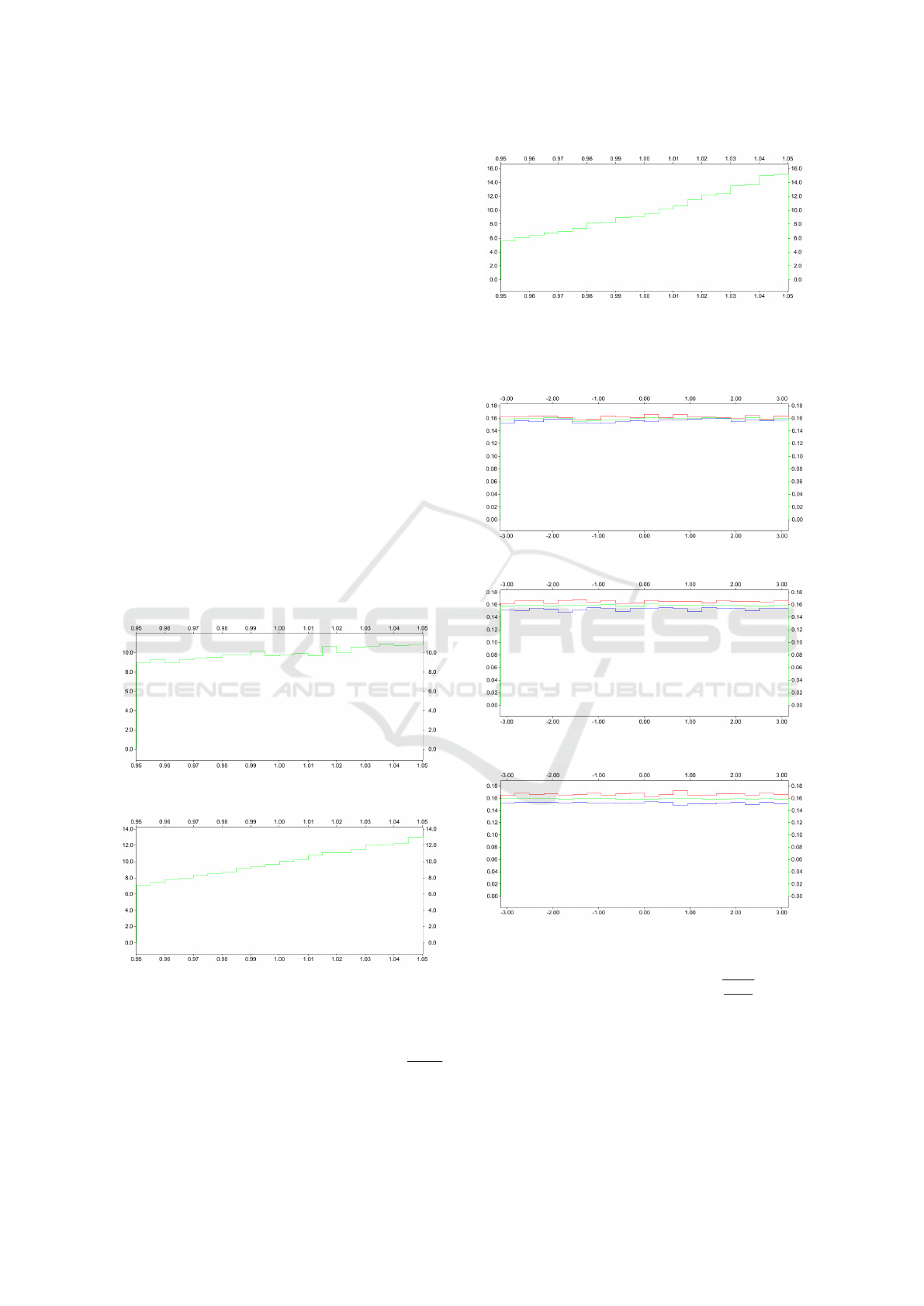
Histograms. For each subcase n ∈ {3, 7, 11}, we
have computed the radius of all samples x and built
the associated histograms (figures 2, 3 and 4) .
Figure 2: (a):Radius histogram (20 divisions); n = 3.
Figure 3: (a): Radius histogram (20 divisions); n = 7.
For each n ∈ {3,7,11} and for all 1 ≤ i < j ≤ n, we
have computed the angle of all samples (x
i
,x
j
) and
built the associated histograms. From these
n(n−1)
2
histograms of each subcase, we have computed the
minimal, mean and maximal histogram. The results
are shown in blue, green and red, respectively, and
Figure 4: (a): Radius histogram (20 divisions); n = 11.
provide an hint on the error of the estimation (fig-
ures 5, 6 and 7) .
Figure 5: (a): Angle histogram (20 divisions); n = 3.
Figure 6: (a): Angle histogram (20 divisions); n = 7.
Figure 7: (a): Angle histogram (20 divisions); n = 11.
By symmetry, the theoretical histograms are uniform.
The errors should be of the order of
q
20
50000
' 0,02 .
In comparison, the errors figured in the angular his-
tograms are quite acceptable, even for the highest di-
mension. The most interesting point is that there is no
rupture in the histogram, which shows that the sam-
pler does manage the subvariety structure. We do not
have an error estimation for the radius histograms.
Simulating a Random Vector Conditionally to a Subvariety: A Generic Dichotomous Approach
117

Actually, the local probability should theoretically in-
crease with the radius, this property being accentuated
with the dimension. This is what is obtained on the
histograms. It is noteworthy however that the sides of
these histograms are subject to additional errors im-
plied by the border of the subvariety.
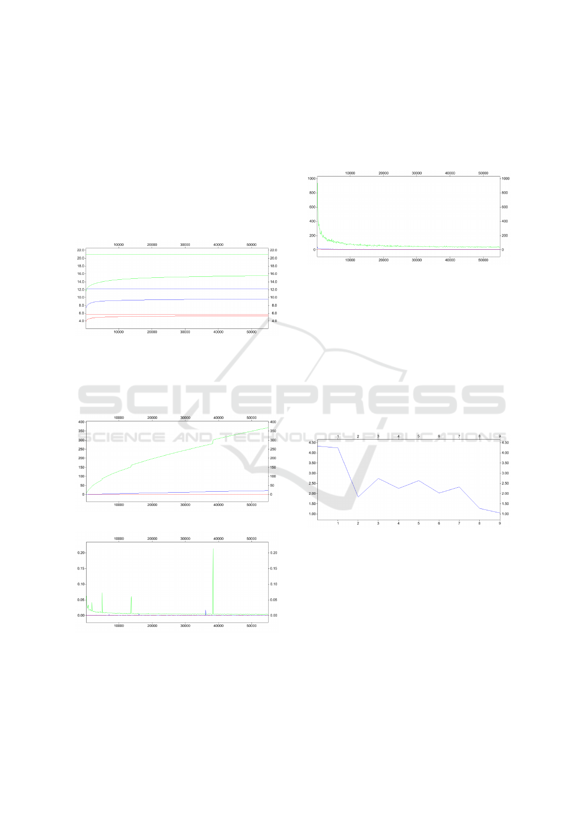
Process Statistics: We present some elements of
measurement on the behavior of the algorithm accord-
ing to the number of generated samples (0 to 55000).
Each figure presents the result for cases n = 3,7,11
with respective colors, red, blue and green.
Figure 8: (a): omg ([b]) versus P(g
a
(X) ∈ []); n = 3, 7,11.
Figure 8 shows how value −log
2
(omg([b]))
evolves and approximates −log
2
(P(g
a
(X) ∈ [])) .
Each curve increases to theoretical value (same color
line), but performance decreases with dimension.
Figure 9: (a): Cumulative cpu time (s); n = 3,7, 11.
Figure 10: (a): Evolution of cpu time (s); n = 3,7,11.
Figures 9 and 10 present the cumulative cpu-time
per thread and the evolution of the cpu-time per sam-
ple and per thread consumed by the process (ex-
pressed in second). The discontinuities in the curves
are caused by intermittent memory allocations. But
we notice clearly that the sampling efficiency in-
creases with the number of generated samples. How-
ever, the cumulative cpu time still increases dramat-
ically with the dimension (the memory use evolves
similarly). Although the curse of dimension has been
delayed by our approach, it is still there.
Figure 11: (a): Evolution of loop retry; n = 3,7,11.
The number of loop retries during the sampling is an
interesting indication of the achievement of the sam-
pling structure (figure 11). It decreases with the num-
ber of samples, and moreover becomes rather small,
even for the highest dimension (around 40 for n = 11).
This result should be compared to the probability of
the subvariety (around 10
−6
for n = 11).
Case b: We present synthetic curves, when the
number of constraints increases. All curves are func-
tion of k, the number of additional constraints. The
values are computed on the 100 last samples.
Figure 12: (b): Evolution of cpu time (ms); k = 0 : 9.
Figure 12 shows the evolution of cpu time per
sample and per thread with k (expressed in millisec-
ond). The curves tend to decrease and approach to
zero. This tendency is not strict however.
Figure 13 presents the evolution of number of loop
retries with k. Again, the tendency is similar. As a
conclusion here, the performance of the sampler is
likely to increase with the number of constraints, and
this is a useful quality.
Case c: On this last test, we computed the radial
histogram and angular histogram (there is only one)
for the samples. These histograms are presented re-
spectively in figures 14 and 15. The quality of the
SIMULTECH 2021 - 11th International Conference on Simulation and Modeling Methodologies, Technologies and Applications
118

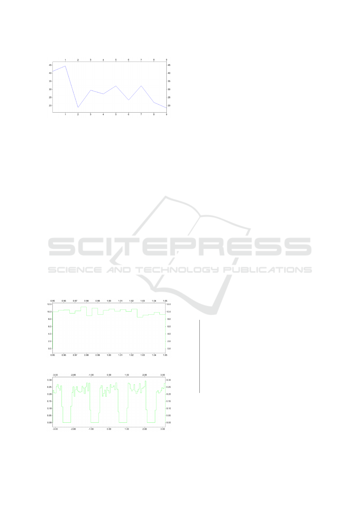
Figure 13: (b): Evolution of loop retry; k = 0 : 9.
histograms is comparable although slightly weaker
than what was observed previously. Due to the con-
straint configuration, the theoretical radius histogram
is uniform, and the theoretical angular histogram is
uniform around each subsegment, A
1
,...,A
4
with a
gradual decrease on the borders. The generated his-
tograms actually comply with these properties.
As a preliminary conclusion, we consider that our
sampling method is globally performant in sampling
conditionally to subvarieties. A future issue will be to
increase the dimension of the sampling space.
4.2 Optimizing a Black-box Function
Such applications to black-box optimization were ac-
tually a great motivation for this work.
Assume that one needs to optimize a function
which is not well known, and which may be com-
puted by a highly costy process (a heavy simulation,
tests made by human teams on the grounds, etc.). Of
course the optimization should be made by sparing at
best the number of calls to the costy evaluation. Is it
possible to solve that? At first sight, it is tempting to
Figure 14: (c): Radius histogram (20 divisions).
Figure 15: (c): Angle histogram (100 divisions).
say no!
In (Jones et al., 1998), Jones, Schonlau and Welch
proposed the efficient global optimization method
(EGO) for addressing such kind of problem. The idea
is to use a surrogate function under the form of a
functional random variable. This functional random
variable is described by means of a Gaussian process
with correlation depending on spatial distance (krig-
ing). Based on such modelling, the construction of
an optimal parameter sequence to be evaluated is ob-
tained by iterating:
• Compute the posterior law of the functional ran-
dom variable, according to the past evaluations,
• Compute the expected improvement function, in
regards to the posterior law and the already best
computed value,
• Choose the parameter optimizing this expected
improvement function and evaluate it.
It is beyond the scope of this paper to detail this semi-
nal work. Whatever, the approach relies on deep sim-
plifications obtained from the Gaussian modelling,
and it tends to be less efficient when the dimension
of the optimization space increases. Works have been
made in order to deal with this dimensional issue;
e.g. (Bartoli et al., 2019). We describe subsequently a
nonlinear interpretation of the EGO method.
A Nonlinear Formalisation. In (Dambreville,
2015), we proposed a nonlinear implementation of
EGO, by considering a (nonlinear) function g(γ,X)
depending on noise model X instead of a kriging-
based surrogate function. The optimal measure
sequence (γ
k
) is obtained by iterating:
1 Function Process next measure
input : γ
j
and g
j
, g(γ
j
,x
o
) for
1 ≤ j ≤ k
output: γ
k+1
and g
k+1
, g(γ
k+1
,x
o
)
2 Make samples of

X


∀ j,g(γ
j
,X) = g
j

3 Compute m
γ
= min
1≤ j≤k
g
j
and:
EI(γ) '
E
X
|
∀ j,g(γ
j
,X)=g
j
min{g(γ,X),m
γ
}
// EI(γ) is approximated from the samples
4 Compute γ
k+1
∈ arg min
γ
EI(γ)
5 Compute g
k+1
, g(γ
k+1
,x
o
)
6 end
By this way, we intend to solve this simple ge-
ometric problem: how to find the isobarycenter γ =
(a,b) of 4 unknown points M
i
= (x
o
i
,y
o
i
) ∈ [−5,5]
2
with i ∈ {1,4} ? The only approach that is possible for
us is to test some solutions by requesting for a costly
Simulating a Random Vector Conditionally to a Subvariety: A Generic Dichotomous Approach
119

measurement; this measurement evaluates function:
g(γ,x
o
) = ||γ − h(x
o
)||
2
, (25)
where h(x
o
) =
1
4
∑
4
i=1
M
i
and x
o
= (x
o
1
,y
o
1
,...,x
o
4
,y
o
4
).
Our purpose is then to optimize (a,b) by doing a min-
imum request to the costly evaluation g(γ, x
o
).
We did not have an efficient method for sampling

X


∀ j,g(γ
j
,X) = g
j

at the time of (Dambreville,
2015). Now, we propose to apply algorithm 3 com-
bined with a discretized method (we actually enumer-
ated on 10
6
discretized points of [−5, 5]
2
) for mini-
mizing the expected improvement EI(γ) in order to
process minimizing sequence (γ
k
) . This sequence
converge to isobarycenter of M
1:4
.
Tests and Results. Points M
1
,...,M
4
are (2, −1),
(3,2), (−
3
2
,4), (
1
2
,3). Their barycenter is (1,2).
We used a sampler with M = 5000, N = 10000 and
[] = [−
1
100
,
1
100
]
k
. Variable X is considered uniform
on [−5,5]
8
. Process is stopped at step k
o
, when op-
timum is found; best evaluation and solution are then
respectively 0 and (1,2). The following table sum-
marizes the results of 100 runs. cpu gives the average
computation time:
k
o
3 4 5
% 46 53 1
cpu(s) 1670 2758 2939
Except for outlier, optimum is found almost
equiprobably after 3 or 4 tries. This is similar to the
geometric method
3
. It is noteworthy that our algo-
rithm does not have geometric knowledge of the prob-
lem and deals with eight dimensions model noise.
5 CONCLUSIONS
We proposed an original dichotomous method for
sampling a random vector conditionally to a subva-
riety. This generic approach, inspired from interval
analysis, is accurate and efficient up to a space of di-
mension 11. We have shown how it could be applied
efficiently to the optimization of expensive black-box
function. The work is promizing from an applica-
tive point of view and offers several improvement per-
spectives. We will particularly investigate some relax-
ations techniques applied to the subvariety in order to
enhance the efficiency of the approach in regards to
higher dimensions.
3
Each measure restricts the solution to a circle. After 2 mea-
sures, we usualy have to choose between two points, and
the solution is found equiprobably at step 3 or 4.
REFERENCES
Abdallah, F., Gning, A., and Bonnifait, P. (2008). Box par-
ticle filtering for nonlinear state estimation using in-
terval analysis. Automatica, 44(3):807–815.
Alefeld, G. and Mayer, G. (2000). Interval analysis: the-
ory and applications. Journal of Computational and
Applied Mathematics, 121(1):421–464.
Bartoli, N., Lefebvre, T., Dubreuil, S., Olivanti, R., Priem,
R., Bons, N., Martins, J., and Morlier, J. (2019).
Adaptive modeling strategy for constrained global op-
timization with application to aerodynamic wing de-
sign. Aerospace Science and Technology, 90:85–102.
Bui Quang, P., Musso, C., and Le Gland, F. (2016). Particle
filtering and the Laplace method for target tracking.
IEEE Transactions on Aerospace and Electronic Sys-
tems, 52(1):350–366.
C
´
erou, F., Del Moral, P., Furon, T., and Guyader, A.
(2012). Sequential Monte Carlo for rare event esti-
mation. Statistics and Computing, 22(3):795–908.
Chabert, G. and Jaulin, L. (2009). Contractor Programming.
Artificial Intelligence, 173:1079–1100.
Dambreville, F. (2015). Optimizing a sensor deployment
with network constraints computable by costly re-
quests. In Thi, H. A. L., Dinh, T. P., and Nguyen,
N. T., editors, Modelling, Computation and Optimiza-
tion in Information Systems and Management Sci-
ences, volume 360 of Advances in Intelligent Systems
and Computing, pages 247–259. Springer.
Dezert, J. and Musso, C. (2001). An efficient method for
generating points uniformly distributed in hyperellip-
soids. In Workshop on Estimation, Tracking and Fu-
sion: A Tribute to Bar-Shalom, Monterey, California.
Jaulin, L., Kieffer, M., Didrit, O., and Walter, E. (2001).
Applied Interval Analysis with Examples in Parameter
and State Estimation, Robust Control and Robotics.
Springer London Ltd.
Jones, D., Schonlau, M., and Welch, W. (1998). Efficient
global optimization of expensive black-box functions.
Journal of Global Optimization, 13:455–492.
Morio, J., Balesdent, M., Jacquemart, D., and Verg
´
e, C.
(2014). A survey of rare event simulation methods
for static input–output models. Simulation Modelling
Practice and Theory, 49:287–304.
Musso, C., Champagnat, F., and Rabaste, O. (2016). Im-
provement of the laplace-based particle filter for track-
before-detect. In 2016 19th International Conference
on Information Fusion (FUSION), pages 1095–1102.
Rubinstein, R. Y. and Kroese, D. P. (2004). The Cross En-
tropy Method: A Unified Approach To Combinatorial
Optimization, Monte-Carlo Simulation (Information
Science and Statistics). Springer-Verlag.
SIMULTECH 2021 - 11th International Conference on Simulation and Modeling Methodologies, Technologies and Applications
120