An Efficient Representation of Enriched Temporal Trajectories
Nieves R. Brisaboa
a
, Antonio Fari
˜
na
b
, Diego Otero-Gonz
´
alez
c
and Tirso V. Rodeiro
d
Universidade da Coru
˜
na, CITIC, Fac. Inform
´
atica, Database Lab. Elvi
˜
na, 15071, A Coru
˜
na, Spain
Keywords:
Compression, Data Management, Trajectories, Correlated Sequences.
Abstract:
We present a novel representation of enriched trajectories of a mobile workforce management system. In
this system, employees are tracked during their working day and both their routes and the tasks performed
at each time instant are recorded. Our proposal tackles the representation of this information paying special
attention to the space footprint without neglecting query time. We performed experiments using real and
synthetic datasets where we show the compression effectiveness as well as the efficiency at query time. Our
results showed that our proposal yields promising results in terms of the space needed to represent both users’
locations and activities while performing access queries to the original data within microseconds.
1 INTRODUCTION
In this modern society, we all rely on devices in or-
der to take part in this entangled dough the globalized
world has become. It has been reported that more than
65% of the adults in advanced economies are owners
of a smartphone but it also stands out that most de-
voted social network users are found in regions with
lower internet rates (Poushter, 2019).
Thus, we are constantly producing a large amount
of data that can be exploited in order to optimize a
wide range of tasks and ease our daily life. Accord-
ingly, an interest for programs able to handle trajecto-
ries and geographical information systems has grown
in recent years giving birth to all kind of algorithms
and systems that are able to locate mobile objects in
real time or recover any past trajectory attending some
user-defined criteria.
The need for studying trajectories not only as a
sequence of time-stamped GPS points but also with a
higher abstraction had led to the appearance of the so-
called semantic trajectories in several works (Moun-
tain and Raper, 2001; Yan et al., 2013; Parent et al.,
2013). Fundamentally, this modern concept defines
a split trajectory where each segment can be classi-
fied into different groups according to a defined pa-
rameter (location, activity, altitude, etc.). After the
segmentation, a semantic label (“visiting a museum”,
a
https://orcid.org/0000-0001-8025-3048
b
https://orcid.org/0000-0001-8263-3298
c
https://orcid.org/0000-0001-6631-4975
d
https://orcid.org/0000-0003-2373-0746
“having lunch at a service area”, “driving through a
traffic jam”, etc.) is assigned to each trajectory seg-
ment (dos Santos Mello et al., 2019). Therefore, se-
mantic trajectories are complex objects composed by
the spatio-temporal polylines of each trajectory and
textual tags identifying the aspect of interest of each
segment.
Even though this approach enables abstract analy-
sis and eases the organization of space-time informa-
tion, there are no standard representations yet. There-
fore, it is an essential need to find a way to store this
vast amount of data (and metadata) following a com-
pact approach to reduce the space footprint without
disregarding the efficient query performance.
Commercial Geographical Information Systems
(GIS) solve this problem by storing all the enriched
segments of a trajectory in a traditional database con-
taining the actual geometry besides all the defining
attributes (semantic tag, initial timestamp, etc.). Des-
pite using some geographical optimizations, GIS so-
lutions can become rather inefficient due to the large
size of the involved tables and its associated cumber-
some handling (Alvares et al., 2007).
In this paper, we propose a novel technique to
store and exploit enriched trajectories to support daily
monitoring in a mobile workforce management sce-
nario. Despite the fact that our proposal is a general-
purpose system that would fit in several domains (e.g.
tourism activities, urban mobility data of vehicles,
etc.), we have defined it as part of a bigger system that
aims at optimizing the daily operation of the work-
ers of an organic-waste management company. One
Brisaboa, N., Fariña, A., Otero-González, D. and Rodeiro, T.
An Efficient Representation of Enriched Temporal Trajectories.
DOI: 10.5220/0010558700490059
In Proceedings of the 10th International Conference on Data Science, Technology and Applications (DATA 2021), pages 49-59
ISBN: 978-989-758-521-0
Copyright
c
 2021 by SCITEPRESS – Science and Technology Publications, Lda. All rights reserved
49

of our main requirements was to supervise employee
tasks in order to gather all possible information to de-
tect any possible malfunction (e.g. if some employees
regularly leave the planned route due to slow traffic it
could be helpful to update the planner system). There-
fore, our work aims to introduce a new structure able
to track the trajectories of employees and the actual
task they were performing at each time instant. As
other works suggest, particularly when movements
are not done in free space, there is no need to store ex-
plicit spatial geometries but only position identifiers
which can be easily geolocated: e.g. segments from a
road network (Brisaboa et al., 2020), rooms inside a
building (Wyffels et al., 2014), etc.
Using this approach, the baseline for our structure
are two correlated sequences that represent the loca-
tion, and the activity done at each time instant by each
user; i.e. one is an ordered list of the road segments
traversed, and the other one is the sequence of activ-
ities performed at each segment (working at a client
place, slow transit on planned route, taking a break,
etc.). Thus, our proposal introduces a unique struc-
ture that represents temporal, spatial, and semantic
knowledge and supports solving queries such as “in-
dicate which tasks were performed by driver X , and
which route did this driver follow to accomplish them
yesterday from 14:30 to 16:00” Also, our system may
solve simpler queries involving a combination of the
associated dimensions; e.g. “where was driver K last
Tuesday at 09:20?” or “what trajectory did driver T
follow this morning?”
2 BACKGROUND
The problem of storing semantic trajectories effi-
ciently has been of interest for more than one decade.
This idea was already tackled in (Schmid et al., 2009)
where a simplified trajectory representation was pre-
sented. In that proposal, they only stored the rele-
vant points of the path through the network along with
inferred timestamps instead of the original trajectory
points.
More recently, a framework that divided trajec-
tories into two separate representations considering
their spatial and temporal components was introduced
(Song et al., 2014). They also proposed a two-stage
error-free spatial compression algorithm and an error-
bounded temporal compression algorithm.
A compressed representation for semantic trajec-
tories was presented in (Gao et al., 2019), where they
used clustering to create regions of interest attending
to those neighboring points that share the same se-
mantic values, and then proposed a hierarchical multi-
resolution network that enables compressing the se-
mantic trajectories as a sequence of semantic regions
of interest.
Meanwhile, the raise of repetitive datasets has led
to the increasing development of compression tech-
niques targeting the exploitation of such repetitive-
ness as a way to reduce their size. Despite the impor-
tance of reducing space, usually this it not the only
concern as compressing data (to reduce their space
needs) is rather useless if a decompression step is
required before querying, as this would slow down
any further exploitation of such data. This spatio-
temporal trade-off is one of the main targets of a
recent research field focused on the development of
compact data structures.
Compact data structures (Navarro, 2016) are a
family of general-purpose data structures that merge
a compressed data representation with efficient query
support. The main advantage of these structures re-
lies on achieving competitive query times while using
almost as little space as in its purely compressed rep-
resentation.
Compact data structures have enhanced all kind
of solutions, from document data mining (Fujishige
et al., 2019) to bioinformatics (Crawford et al., 2018).
In the scope of this work, there are some previ-
ous works tackling trajectory representations through
compact data structures. Among them, an efficient
representation for trajectories in free space was pro-
posed in (Brisaboa et al., 2019). Using a system based
on snapshots that store the positions of the objects
at some (regular) given time instants and additionally
keeps their relative movements between two consecu-
tive snapshots, they are able to solve a range of spatio-
temporal queries based on the movement of objects in
a grid. A multidimensional representation for han-
dling event sequences has also been proposed in the
area of semantic trajectories (Brisaboa et al., 2018).
That work presents a data reorganization strategy that
aims at grouping/ordering the information of interest
attending one (or several) of its semantic tags, and
leads to an efficient representation to solve aggrega-
tion queries.
Figure 1: A bitvector B and its two operations: rank and
select.
One common basic component of these structures
are bitvectors (or bit sequences). A bitvector B[1, n]
is a sequence of zeros and ones of length n, where
the following two basic operations (also depicted in
DATA 2021 - 10th International Conference on Data Science, Technology and Applications
50

Figure 1) are expected to be supported:
• rank
1
(B,i) returns the number of bits set to
1 in B[1..i]. Alternatively, rank
0
(B,i) = i −
rank
1
(B,i). Note that B[i] = rank
1
(B,i) −
rank
1
(B,i − 1).
• select
1
(B,i) returns the position in 1..n where the
i-th 1 occurs. Therefore, rank
1
(B,select
1
(B,i)) =
i.
Similarly, operations rank
0
(B,i) and select
0
(B,i)
can be defined to respectively count the number of
zeros up to a given position, or locating the position
in B of the i-th zero.
Compressed bitvector representations exist (Ra-
man et al., 2002; Okanohara and Sadakane, 2007;
Navarro, 2016). However, in this work we have
used plain bitvectors with select and rank support,
achieving both operations a time complexity of O(1)
by using just o(n) additional bits of space (Munro,
1996). Besides, we have used a special operation
known as selectNext
1
to speed up consecutive select
1
queries (Navarro, 2016). Basically, if B[i] contains a
one, j = selectNext(B, i) returns the position j ( j > i)
of the next one in B.
Despite the good computation properties bitvec-
tors offer, compact data structures rely on some com-
pression methods to effectively store the non-binary
information. One of the most popular compression
algorithms used in the context of repetitive datasets is
Re-Pair (Larsson and Moffat, 1999). This algorithm
exploits pair repetition on a sequence relying on a dic-
tionary of rules. Basically, each pair of symbols oc-
curring at least twice is substituted by a new symbol,
hence shortening that sequence. In addition, a rule re-
lating both the pair and the new symbol is created to
allow further decompression. Re-Pair algorithm pro-
ceeds as follows:
• The most frequent pair xy in a given sequence T
is located.
• A new rule X → xy is created and stored in a dic-
tionary of rules D.
• Each occurrence of the original pair is replaced in
T by X .
• The previous three steps are repeated recursively
until there are no repeated pairs in T .
As an example to illustrate the behaviour of Re-
Pair, let us consider the sequence T = honabonanai
and D =
/
0, we can see that the most common pair
of symbols in T is na. Thus, the algorithm gener-
ates a new rule R
1
: A → na, which is added to the
dictionary D, and replaces all the occurrences of na
in T by A. The resulting sequence now becomes
T
0
= hoAboAAi, and D = {R
1
: A → na}. This pro-
cess is repeated recursively until the text contains no
more repeated pairs. In our example, the next gen-
erated rule is R
2
: B → oA, transforming the text into
T
00
= hBbBAi, and D = {R
1
: A → na; R
2
: B → oA}.
The algorithm ends due to the lack of repeated pairs.
3 OUR PROPOSAL
As stated before, the main idea of this work arises as
part of a real mobile workforce management system
in the scope of a organic-waste handling company
where not only the trajectories of their employees
are of interest but also the activity performed by
them at each spatio-temporal point. Since the
range of possible daily tasks performed by waste
management truck drivers is very restricted, we were
able to reduce the list to only 8 activities: being
at headquarters, visiting a customer place, taking a
break, normal/slow driving on un/planned route, and
inactive. Thus, our problem can also be seen as the
search for an efficient representation able to associate
each segment traversed by a worker during his daily
trajectory with one of those tasks.
A
A
A
A
A
A
A
C
C
C
C
C
C
C
C
C
D
X
X
X
X
Y
Y
Y
Z
Z
Y
Y
Y
Y
Y
Z
Z
Z
A:
R:
1
0
2 3 4 5
6
7
8
9 11
10
12 13 14 15 16
Figure 2: Original representation of both correlated se-
quences: road segments traversed (R) and activities per-
formed (A).
A straightforward (naive) approach of our pro-
posal would be to handle two aligned vectors contain-
ing the value of each dimension during a discretized
time period, as depicted in Figure 2. Therefore, we
would have a vector R saving the identifiers of the
road segments traversed by an employee and a sec-
ond vector A containing the activities performed by
the worker. As the company tracks both values at ev-
ery minute thanks to the driver’s mobile phone, each
element in both sequences represents a time interval
of 60 seconds.
This naive solution contains a high degree of re-
dundancy that can be exploited for the sake of com-
pression. Given that each symbol in the previous se-
quences is represented with an integer identifier, it is a
priority to reduce the number of repeated symbols of
a sequence. This can be achieved with what we call
a header vector, that is, a vector which avoids con-
secutive repeated symbols as R
H
in Figure 3. Using
only this header vector it would be possible to retrieve
An Efficient Representation of Enriched Temporal Trajectories
51

the route followed by a worker on the actual chrono-
logically ordered sequence of activities an employee
has completed in a day. However, recall that the naive
representation keeps the ordered sequence of events
and, through consecutive repetitions, how much time
was spent in each location/activity. This information
would not be kept by storing just R
H
(or A
H
for activ-
ities) as indicated in Figure 3. In order to retain this
feature the header vector needs to be complemented
with a bitvector B representing each time interval as in
the naive solution. Thus, as depicted in Figure 3, R
H
contains the actual information of each event change
while B just ticks every time interval j and whether it
corresponds to a new event of the header vector (B[ j]
set to 1) or it is just a repetition of the last one (B[ j]
set to 0). Note that to recover R[8] = C from Figure 2,
we have to count how many ones are there up to posi-
tion 8 in B, i.e. we compute rank
1
(B,8) = 2, and then
access the second position of R
H
; i.e R
H
[2 − 1] = C.
A
A
A
A
A
A
A
C
C
C
C
C
C
C
C
C
D
X
X
X
X
Y
Y
Y
Z
Z
Y
Y
Y
Y
Y
Z
Z
Z
A:
R:
1
0
2 3 4 5
6
7
8
9 11
10
12 13 14 15 16
1 0 0 0 0 0 0 1 0 0 0 0 0 0 0 0 1
A
C
D
R
H
:
1
0
2
B:
1
0
2 3 4 5
6
7
8
9 11
10
12 13 14 15 16
Figure 3: Example illustrating how we can decrease the
space needs of R, by using R
H
and a bitvector B.
It is important to note that we work with two cor-
related sequences R and A in our particular context,
so we need to store information about both sequences.
Keeping in mind the idea of reducing space, instead
of using two header vectors and two bitvectors, we
can store two header vectors R
H
and A
H
and only
one smaller structure to determine symbol repetitions.
The main problem we have to deal with by following
this approach, is that we have to be able to quickly
identify changes in each sequence and, particularly,
changes that occur simultaneously (in both sequences
at the same time). To tackle that, we use a bitvec-
tor identifying a transition (in activities, trajectories
or both) and, at least, another bitvector to discriminate
which sequence has changed. In order to achieve this
purpose, we introduce three different bitvector-based
solutions:
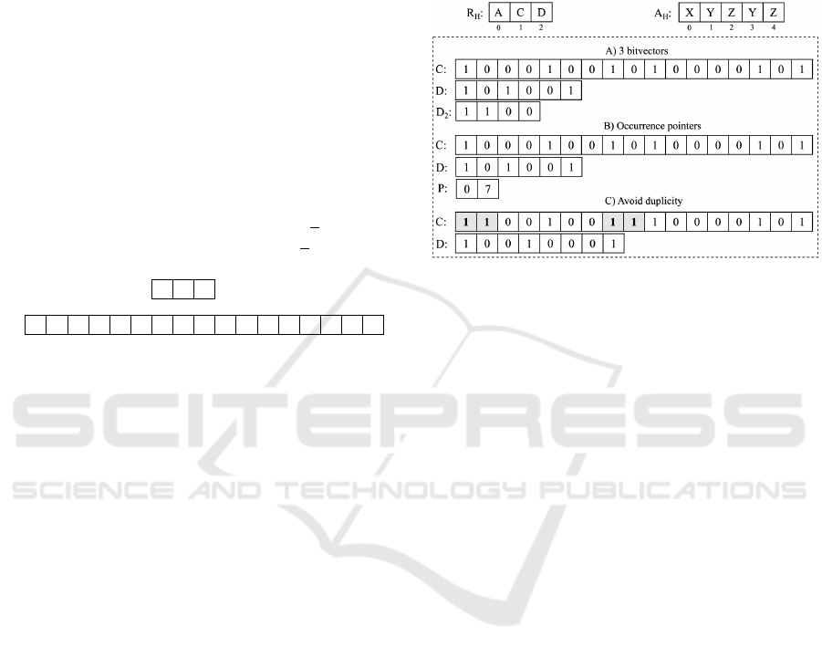
• 3 Bitvectors (3B): This approach uses three
bitvectors to detect changes in both sequences.
The first bitvector (C) identifies change events in
any vector. The second bitvector (D) discrimi-
nates between single changes in vector R (with
greater change probability). Last bitvector (D
2
)
differentiates between single changes in sequence
A and double changes (in both R and A) at the
same time instant.
• Occurrence Pointers (OP): This solution shares
the same bitvector C to identify changing time in-
stants in both vectors R and A, and uses D to dis-
cern which sequence has changed. The events of
double changes at the same instant are handled
with a new array P that keeps pointers to the orig-
inal positions (within C) where they occurred.
Figure 4: Our proposal uses two common arrays (R
H
and A
H
) to store three dimensional information (including
time), one bitvector C to encode changes on them and one
of the three types of auxiliary structures to manage two-
dimensional changes in C.
• Avoid Duplicity (AD): A simpler lossy method to
tackle the concurrent changes problem would be
to force them into different time instants. Thus,
each double change event would be represented
in C as two consecutive changes, assigning in D
vector a one to each. It is important to notice that
this approach may imply some inaccuracies that
would translate into loss of detailed information
due to the lack of a third level. In a context where
this could become a usual issue, the fix could con-
sists in using a finer granularity, i.e. to survey ac-
tivities and locations every second instead of ev-
ery minute so that double changes would become
very unlikely.
3.1 Handling Drivers’ Work Shifts
The above proposals permits us to handle the activi-
ties and locations of any given employee. However,
our aim is to represent a complete dataset with the
information corresponding to all the existing drivers
along a large period of time of K working days.
Therefore, our bitvectors C, D, D
2
, and vector P could
contain information corresponding to different drivers
during up to K distinct days, and we have to be able
to distinguish which part of those structures belongs
to each driver and day.
We use a little auxiliary structure in order to check
the working days when each employee worked, as not
DATA 2021 - 10th International Conference on Data Science, Technology and Applications
52

all drivers work every day. In particular, we use a
chronologically ordered bitvector dxc containing K
bits for the first driver, other K bits for the second
driver, and so on, where a 1 indicates that an employee
worked a given day, and 0 means the opposite.
1 1 0 0 1
R:
0
K = 5
dxc:
0 1 0 1 0
1
K
1 1 0 1 1
2
K
0 1
2
3 4
5
6 7
8
9
10 11 12
13
14 15
16
17
18
19
20
21
22
23
24 25
26 27
28 29
30
31 32
33 34
35
A:
0 1
2
3 4
5
6 7
8
9
10 11 12
13
14 15
16
17
18
19
20
21
22
23
24 25
26 27
28 29
30
31 32
33 34
35
C:
0 1
2
3 4
5
6 7
8
9
10 11 12
13
14 15
16
17
18
19
20
21
22
23
24 25
26 27
28 29
30
31 32
33 34
35
it=4
1
0
2 3 4
5
6
7
8
9
11
10
12
13
14
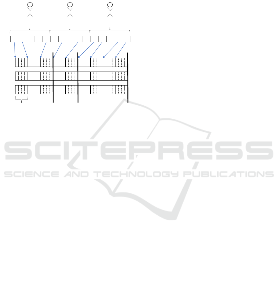
Figure 5: Bitvector dxc identifies the days on which drivers
have worked and enables easy acces to the corresponding
offsets in road segments vector (R), activity vector (A) and
changes vector (C).
In practice, our auxiliary bitvector acts as an ar-
ray of pointers to the initial position of a workday of
a given driver in vectors R, A and, C. In dxc, each
driver has the same amount of workable days K, and
each of those days is divided into a constant amount
of discretized time intervals it. Therefore, it can be
easily checked if a given driver worked on a given
day by computing w = dxc[(driver ∗ K) + day − 1].
If the employee worked that day (w = 1), the off-
set in R (and also in A and C) for this driver on
that day can be obtained by accessing from position
l = it ∗ rank
1
(dxc, (driver ∗ K) + day − 1) to posi-
tion r = l + it − 1. We define an operation [l,r] ←
getRange(dxc, driver,day) accordingly.
As an example, let us consider Figure 5, where
we store information for K = 5 days and, for each
day, we handle it = 4 time intervals. We can check if
driver 1 worked on day 2 as w = dxc[(1∗ 5)+2 −1] =
dxc[6] = 1. Once we have confirmed that the driver
worked on that day, we can jump directly to the
range defined by position l = 4 ∗ rank
1
(dxc, 6) = 12
in R (also for A or C), and r = 12 + 4 − 1 = 15.
This range can be obtained directly as [12,15] ←
getRange(dxc, 1,2), as defined above.
3.2 Reducing Space Usage
In the particular context of a mobile workforce man-
agement system, there will always be intrinsic global
repetitiveness not considered in the previous section.
Previously, we have defined some techniques to ex-
ploit symbol repetitions during a given workday of
a single employee, i.e. we take advantage of long
periods where a worker performed the same activity
or traversed the same road/highway. However, if we
analyze the behaviour of several employees globally,
we may find again a high degree of repetitiveness be-
tween them. For example, examining the trajecto-
ries of every worker, it seems quite likely that they
always start the route at headquarters and then tra-
verse the same streets/roads (or at least a reduced set
of them). The same applies to activities, it is expected
that workers perform the same activity sequence, e.g.
a driver leaves the planned route due to a traffic jam.
As detailed in Section 2, Re-Pair is a compression
technique that exploits global repetitions. Expected
that, by applying Re-Pair over our header vectors R
H
and A
H
, we could be able to reduce their memory
footprint even further, yet probably in exchange for
a slower access time. Note that if we have R
H
and A
H
compressed with Re-Pair, each time we wanted to ac-
cess any of their elements, we would have to decom-
press them from the Re-Pair compressed sequence.
4 QUERIES
We have selected four representative queries to show
how our structure (considering its three variants 3B,
OP, and AD) works. On the one hand, we offer ac-
cess capabilities for routes and activities (RouteAt-
Time and ActivityAtTime); i.e. recovering the corre-
sponding location/activity of a particular driver at a
given time instant. On the other hand, we provide
temporal window queries for both dimensions (Route-
sAtTimeRange and ActivitiesAtTimeRange).
• RouteAtTime (RT): This query recovers the road
segment identifier where a driver was in a specific
instant; i.e. it permits us to obtain the location of
any worker at a given time instant.
It takes three input parameters: driver, day, and
time
instant. Thanks to the already explained cal-
culations on the bitvector dxc (see getRange op-
eration in Section 3.1) we can obtain the positions
[l,r] within bitvector C that correspond to the in-
formation regarding the given day of a particular
driver. Recall that range of positions is obtained
as [l,r] ← getRange(dxc,driver,day).
An Efficient Representation of Enriched Temporal Trajectories
53

Then, using the parameter time instant we can get
the position I = l + time instant of the queried
time instant within the day. The number (S) of
ones in bitvector C until the position I (computed
as S = rank
1
(C,I)) represents the total number of
time instants when there were changes (routes and
activities) until the time instant of interest. That is,
changes within R[0,I] or A[0,I].
As explained before, bitvector D allows to dis-
criminate routes information. Thus, we can easily
obtain the total amount of road segment changes
until the queried instant as J = rank
1
(D,S).
Therefore, J − 1 represents the position on R
H
where the road segment identifier is stored.
• RoutesAtTimeRange (RTR): This query recon-
structs the trajectory of a driver for a specific in-
terval of time. With this query we are able to ob-
tain the driver‘s route in a given working day. It
takes three input parameters: driver, day, and an
interval time [X..Y ].
We can use the previous query to find the first road
segment identifier of the queried interval [X ..Y ]
by just computing RouteAtTime(driver,day,X).
During that process, recall we obtain the corre-
sponding position I within C, and S = rank
1
(C,I)
within D corresponding to the last road change
that occurred either before or at time instant X.
However, in order to retrieve the full trajectory
of a driver during the given interval, we need
to traverse the ones within D from S on using
selectNext
1
(D,S); i.e. jumping to the following
road segment changes marked on D. Note that
this process must end once we have gone further
than the corresponding position E = I + (Y − X)
associated to Y in C.
Therefore, we start with the same I
and S = rank
1
(C,I) values obtained by
RouteAtTime(driver, day,X), and also output
the (initial) road segment identifier within
R
H
[rank
1
(D,S) − 1] n times, where n =
selectNext
1
(D,S) − S − 1. Then, while it holds
that I ≤ E, we set n = selectNext
1
(D,S) − S − 1;
S = selectNext
1
(D,S) (hence looking for the next
road segment change in D); we output the road
segment identifier in R
H
[rank
1
(D,S) − 1] n times;
and finally compute I = select
1
(C,S) to map the
position S from D into C, which allows us to
know if the process must either end (I > E) or
handle the next road-segment change otherwise.
• ActivityAtTime (AT): This query allows us to re-
turn the activity being performed by a driver at a
specific instant. It takes three input parameters:
driver, day, and time
instant.
This query is rather similar to RouteAtTime but
instead of just using bitvectors C and D, this time
it will be necessary to reach the deepest bitvectors.
Recall that Section 3 already introduced our three
strategies to deal with double changes (road seg-
ment and activity changing at the same instant).
We can get the position in D as we did in the pre-
vious queries (recall how S and I were initialized
for RouteAtTime operation). However, D does not
discriminate between activity identifiers and dou-
ble changes, and here is where our alternatives
differ:
– 3 Bitvectors (3B): Uses a third bitvector D
2
to
be able to compute if the i-th one in D corre-
sponds only to a road segment change (D
2
[i] =
0) or to a double change (D
2
[i] = 1). It is im-
portant to note that, for this query, this alter-
native needs to consider single activity changes
(zeros in D) and double changes (ones in D
2
)
up to position S (where S was the position in
C associated to the time instant of interest).
Therefore, the amount of double changes can
be computed as DC = rank
1
(D
2
,rank
1
(D,S)),
while single activity changes can be counted as
AC = S − rank
1
(D,S). Finally, DC + AC gives
us the total amount of activity changes until the
queried time instant. Thus, we obtain the activ-
ity being performed by the given driver at the
indicated time instant by accessing the value
A
H
[DC + AC − 1].
– Occurrence Pointers (OP): In this solution we
use a list of pointers P pointing at the posi-
tion of ones in C which correspond to a double
change.
To obtain the total number of simultaneous
changes DC up to the position I from C, we
count all the values of P that are below I (us-
ing a binary search over P that takes O(log |P|)
time, to locate the last index p such that P[p] ≤
I). The single activity changes can be obtained
as AC = rank
0
(D,S). Concluding again that the
driver was performing activity A
H
[DC + AC −
1].
– Avoid Duplicity (AD): This solutions un-
folds simultaneous changes in two consecu-
tive single changes, significantly simplifying
the operations. Hence, the total amount of
activity changes until the queried time in-
stant can be obtained by simply computing
AC = rank
0
(D,S) and the searched activity is
A
H
[AC − 1].
DATA 2021 - 10th International Conference on Data Science, Technology and Applications
54

• ActivitiesAtTimeRange (ATR): This query al-
lows us to return the sequence of activities of a
given driver during a particular time interval. It
also takes three input parameters: driver, day, and
an interval time [X..Y ].
This query is rather similar to
RoutesAtTimeRange, yet returning a list of
activities instead of road segments. Therefore,
as is the case with ActivityAtTime, it will be
necessary to traverse the deepest bitvectors.
Again, we can calculate the initial position S in
D discriminating the activities from the double
changes as it has been explained before for oper-
ation ActivityAtTime. Then, each alternative rep-
resentation will retrieve the list of activities in a
different way:
– 3 Bitvectors (3B): As usual, the first activity
identifier to return can be computed with
ActivityInTime(driver,day, X), along with I
and S positions that are obtained as in the
previous explanations. Again, this alterna-
tive needs to check single activity changes
(zeros in D) and double changes (ones in
D
2
). Therefore, the position of the next single
activity change after S, may be calculated
as AC = selectNext
0
(D,S), while the next
double change would be at position DC =
select
1
(D,selectNext
1
(D
2
,rank
1
(D,S))).
Thus, the first activity of interest
was performed during the interval
C[I,select
1
(C,min(DC,AC)) − 1]; i.e. it must
be output n = select
1
(C,min(DC,AC)) − I − 1
times. Then, the next activity in A
H
starts,
so we update I = select
1
(C,min(DC,AC)),
compute the new AC and DC positions to
obtain again the smallest value, and the
process would be repeated until we have
gone further than the corresponding position
E = I + (Y − X) associated to Y in C (as in
RoutesAtTimeRange).
– Occurrence Pointers (OP): To get the
value of the first activity change in the
time interval [X..Y] we use the query
ActivityInTime(driver,day, X). Then, AC
can be computed as in the previous alternatives
(using selectNext
0
in D) while DC would be the
amount of all the pointers P[i] that fall within
the queried interval [rank
1
(C,I),rank
1
(C,E)].
– Avoid Duplicity (AD): Due to the simplic-
ity of this alternative, the calculations are
practically the same as RoutesAtTimeRange
but this time operating over activity changes
(zeros); hence, traversing D at positions S, S
0
=
selectNext
0
(D,S), and so on.
5 EXPERIMENTAL EVALUATION
This section describes the two datasets (one for route
identifiers and another one for activity identifiers) that
have been used to test our structure in terms of com-
pression effectiveness and performance at query time.
We analyze the results obtained, comparing the three
variants of our proposal. Finally, Section 5.2.3 in-
cludes our experiments to show the results obtained
when Re-Pair is applied on the header vectors R
H
and
A
H
.
5.1 Datasets
We can distinguish two types of datasets used along
this work: one real dataset that consists of the po-
sitions of the employees of our collaborating com-
pany during their workday, and two synthetic activity
datasets to test different scenarios.
The first one was obtained from the GPS data
stored by the mobile phones of the truck drivers dur-
ing their routine gathering waste and, essentially, it is
a chronologically ordered list of road segment iden-
tifiers that are recorded at discretized time intervals
of 60 seconds. The resulting number of entries in R
was 14,439,424 and the number of different road seg-
ments handled was 101,623.
The second type of datasets are synthetic datasets
that we generated due to the lack of real activity
data. Using the 8 activities described in Section 3,
we designed these synthetic datasets resembling nor-
mal employees behavior as much as possible. To en-
sure the realism of this data, we developed a complex
system where each road segment is assigned a sub-
set of possible activities based on its geolocation (e.g.
the activity “being at headquartes” cannot be possible
outside the company facilities). Since we were gen-
erating the activities associated to each driver along
each road segment present in R, the number of entries
in A was also 14,439, 424.
With the aim of testing a wide range of scenarios
we created two activity datasets attending to differ-
ent degrees of variability. Note that the behaviour of
our proposal may differ depending on the amount of
activity changes (both, compression ratios and access
times). We created two activity datasets: one with a
low rate of variability (there is a change in the value
of the activity every 100 instants of time) and another
dataset with a higher variability (there is a change in
the value of the activity every 10 instants of time).
An Efficient Representation of Enriched Temporal Trajectories
55

5.2 Experimental Results
We have run experiments using the three variants
of our proposal (3B, OP, and AD) to compare their
compression effectiveness and performance to ac-
cess the original information. Our experiments were
run on an isolated computer using an Intel Xeon
ES2470@2.30GHz processor (20 MB of cache) and
64 GB of RAM. It runs Debian 10.8 (buster) with ker-
nel 5.4.0 (64 bits). The compiler used was g++ ver-
sion 7.4.0, with C++17 option (-std=c++17).
As a baseline for our comparison we have im-
plemented the naive solution depicted in Figure 2.
This simple approach uses just two symbol sequences
(road segment identifiers and activity identifiers).
To make this proposal more competitive in terms
of space needs, we have chosen an efficient bit-
compaction representation for these sequences, in
which all identifiers are stored using the minimum
number of bits b needed to represent the maximum
value of the vector u (i.e. b = dlog
2
ue bits). Our
bit-wise compacted vectors for A and R were imple-
mented using the SDSL library (Gog et al., 2014). Re-
call that since the number of different road segments
is 101,623 we used only b = 17 bits per road segment
identifier. Similarly, since we had only 8 different ac-
tivities, 3 bits per activity identifier were used. Conse-
quently, the overall size of the baseline representation
of the sequence R was 30.7 MiB, while for sequence
A we used 1.8 MiB, totalizing 32.5 MiB.
The same bit-wise compaction strategy was also
applied to our proposal, where both header vectors,
R
H
and A
H
, were stored using bit-wise SDSL vectors.
5.2.1 Compression Results
As stated before, synthetic activity datasets were used
to test our proposal under different scenarios with two
different degrees of repetitiveness (higher or lower
amount of consecutive repeated values).
Table 1: Compression ratios as % of the baseline represen-
tation using the activity dataset with a low repetitiveness
(one change every 10 activities).
3B OP AD
26.69 32.24 26.40
Table 1 shows how the space needs
1
of our three
alternative representations using an activity dataset
with low repetitiveness (activities change once every
1
We show compression ratio as the percentage of the size
of the compressed representation (c) with respect to the
baseline representation (s) of the source data; i.e. 100 ×
c/s.
10 activities). As we can see, the best compression
results are obtained by the AD solution (26.40%), fol-
lowed closely by 3B (26.69%). On the other hand,
the pointer vector of OP negatively affects its space
footprint (32.24%).
Table 2 depicts the compression ratios for our pro-
posals but this time using an activity dataset with high
repetitiveness ratio (activities change once every 100
activities). AD is still the most compact approach, but
now results are much more similar because, with that
low rate of activity changes, it is less likely a double
shift to occur, i.e. third level vectors (D
2
in 3B and P
in OP) contain little data.
Table 2: Compression ratios as % of the baseline represen-
tation using the activity dataset with a high repetitiveness
(one change every 100 activities).
3B OP AD
11.71 11.71 11.48
Comparing the results in Tables 1 and 2, we can
see that the behaviour of our proposal is far better
when applied to a repetitive scenario. This is mainly
due to the fact that increasing the number of con-
secutive repeated values allows our proposal to re-
duce significantly the header vectors sizes. This also
affects the bitvectors of our proposed variants since
with a higher amount of consecutive repetitions the
bitvectors C and D (see Figure 4) may become sparse
bitvectors.
5.2.2 Access Time Results
With the aim of analyzing access time to our proposed
structures we have tested the queries described in Sec-
tion 4. We compared the querying time obtained by
the baseline representation with that of our three pro-
posed alternatives. Again, all experiments were car-
ried out using a real route dataset and two synthetic
activity datasets.
Regarding route queries (RT and RTR), the first
consideration we should note is that our three alter-
natives use roughly the same amount of time for both
queries as all three solutions share the same underly-
ing computation, that is, there is no need in any pro-
posed alternative to reach the deepest vectors.
Table 3: Access times (ns) for route information.
Baseline 3B OP AD
RTR 90.0 100 100 100
RT 0.50 10 10 10
Table 3 depicts how our solutions are not far from
the baseline when accessing the road segments tra-
DATA 2021 - 10th International Conference on Data Science, Technology and Applications
56

versed by a driver during a (random) complete day
that involves 600 minutes (RT R). However, we are
not so competitive when we perform an access (RT )
to retrieve the road segment identifier corresponding
to a unique (random) time instant. In the latter, the
baseline is capable of accessing any position of any
vector in constant time, while our proposal needs to
map the queried position in the header vector through
the different bitvectors.
Concerning activities, query times corresponding
to operations AT and ATR become worse because our
proposal needs to roam deeper in our bitvector hierar-
chy. However, it is important to keep in mind that our
structure may use up to 88% less space than the orig-
inal representation. Tables 4 and 5 include the results
obtained for our two synthetic activity datasets.
Table 4: Access times (ns) to the activity dataset with a low
repetitiveness (one change every 10 activities).
Baseline 3B OP AD
ATR 90.00 200 210 180
AT 0.70 98 165 90
A lower degree of repetitiveness (i.e. having
a large amount of activity changes) affects directly
the amount of information stored in our proposal as
header vectors increase proportionally and, conse-
quently, the amount of ones stored in our bitvectors
grows accordingly. This largely worsens AT R access
times as the efficiency in our proposed bitvectors de-
pend on the ability to jump between consecutive ones,
skipping a huge amount of 0’s.
Table 5: Access times (ns) to the activity dataset with a high
repetitiveness (one change every 100 activities).
Baseline 3B OP AD
ATR 90.00 120 140 110
AT 0.70 30 50 13
Nonetheless, Table 5 shows that query times for
AT R become more competitive when a highly repet-
itive dataset is used, although we are still clearly
slower than the baseline representation at AT access
queries.
Regarding the three different alternatives of our
proposal, AD is still the fastest variant as it has one
less level to traverse during the query.
5.2.3 Applying Re-Pair
We applied Re-Pair over R
H
and A
H
sequences in our
proposals as a way to exploit the expected underly-
ing repetitiveness within them. We can see below that
we obtained an improved compression ratio. How-
Table 6: Compression ratios (in %) using Re-Pair on the
activity dataset with a low repetitiveness ratio (one change
every 10 activities).
3B OP AD
98.55 116.67 97.78
ever, access times largely worsened due to the need
of performing a Re-Pair decompression process from
the beginning of the sequence to recover the original
data.
In practice, to provide pseudo-random access to
the compressed data we enriched our Re-Pair imple-
mentation with a list of pointers referencing the be-
ginning of each day. This provided synchronization
points at the beginning of each day and consequently
sped up the partial decompression of our sequences
R
H
and A
H
as a full decompression was no longer
necessary.
Table 7: Compression ratios (in %) using Re-Pair on the
activity dataset with a high repetitiveness (one change every
100 activities).
3B OP AD
88.68 86.79 86.79
Tables 6 and 7 present the compression ratios af-
ter applying Re-Pair in our solutions. For the sake of
a fair comparison, all the results presented in this sec-
tion have been measured against a compressed base-
line using the same enriched Re-Pair algorithm. Note
that, while the previous baseline required 30.7 MiB,
our new baseline compressed with Re-Pair required
13.8 MiB in the lesser repetitive scenario and 5.3 MiB
in the higher repetitive one. Therefore, Re-Pair was
surprisingly successful in the non-repetitive scenario,
where we could decrease the space requirements of
the regular uncompressed baseline to around 44.9%
of its size. In the most repetitive scenario, using
Re-Pair led to even better results, reducing the space
needs to around 17.2% of the original size.
Firstly, Table 6 details the Re-Pair compression re-
sults obtained for the lesser repetitive activity dataset.
We can see that the results obtained by our proposals
hardly improve the values of the baseline represen-
tation, and indeed, in the variant OP, space require-
ments are worsen than those of the baseline. Sec-
ondly, Table 7 describes a slightly better scenario re-
garding the high repetitiveness dataset as all our al-
ternative representations overcome the results of the
baseline.
The cost of reducing the space requirements is
paid at query time because, as indicated above, par-
tial decompression is required. Access time typically
worsens by a constant factor F of roughly around
An Efficient Representation of Enriched Temporal Trajectories
57

Table 8: Access times (ns) to the route dataset with Re-Pair.
Baseline 3B OP AD
RTR 3090 3100 3100 3100
RT 3001 3010 3010 3010
3000 nanoseconds (see Tables 8, 9, and 10) corre-
sponding to the decompression of either 600 road seg-
ments identifiers (RTR) or 600 activity values (ATR).
Note that, for RT and AT, we are also paying that ex-
tra decompression cost because, in our current imple-
mentation, we are decompressing all the 600 values
corresponding to a day, even though we are just re-
trieving one of those values. This is clearly and un-
optimized operation that we will improve shortly by
partially decompressing up to the queried time instant
of the day.
Table 9: Access times (ns) to the activity dataset with a low
repetitiveness ratio (one change every 10 activities) with
Re-Pair.
Baseline 3B OP AD
ATR 3090 3200 3210 3180
AT 3001 3110 3165 3090
Again, apart from the extra decompression cost,
the results obtained by our variants are similar to
those in the previous sections where Re-Pair was not
used.
Table 10: Access times (ns) to the activity dataset with a
high repetitiveness (one change every 100 activities) with
Re-Pair.
Baseline 3B OP AD
ATR 3090 3120 3140 3110
AT 3001 3040 3060 3025
To sum up, we can see that, as expected, using Re-
Pair brings a space/time trade-off. We save space, yet
our solution becomes clearly slower at query time.
6 CONCLUSIONS AND FUTURE
WORK
We have presented a novel representation of en-
riched trajectories as part of a real mobile work-
force management system. Our proposal includes
three variants, where each of them employs a differ-
ent bitvector-based solution in order to achieve a good
trade-off between spatial footprint and query times.
Our proposal has been tested against real and syn-
thetic datasets, using different distributions in the lat-
ter in order to study the behaviour of our proposal
in diverse scenarios. Experiments have shown how
our new representation is able to store large amounts
of information using around a 88% less space than
our baseline technique while obtaining competitive
access times.
In addition, we have analyzed the use of a well-
known compression technique, known as Re-Pair, to
boost the already good compression ratios achieved.
Our experiments showed Re-Pair was able to reduce
the size of our proposal even further, at the cost of
slower access times.
As future work, our main aim would be to create
another compression representation that could allow
reduce even further the space requirements while re-
taining good performance at query time. Apart from
that, we are also working on endowing our proposal
with dynamic capabilities, i.e. enabling the informa-
tion stored in it to grow over time.
ACKNOWLEDGEMENTS
Partially funded by the CITIC research center funded
by Xunta/FEDER-UE 2014-2020 Program, grant
ED431G 2019/01.
MICIU (PGE/ERDF) [Datos 4.0: TIN2016-78011-
C4-1-R; STEPS: RTC-2017-5908-7; BIZDEVOPS:
RTI2018-098309-B-C32].
IGAPE/Xunta (FEDER-UE) 2014-2020
[IG240.2020.1.185].
Xunta/GAIN (ERDF) [GEMA: IN852A 2018/14]
and by FPI Program [BES-2017-081390].
REFERENCES
Alvares, L. O., Bogorny, V., Kuijpers, B., de Mac
ˆ
edo, J.
A. F., Moelans, B., and Vaisman, A. A. (2007). A
model for enriching trajectories with semantic geo-
graphical information. In Proceedings of the ACM
International Symposium on Geographic Information
Systems, ACM-GIS 2007, page 22.
Brisaboa, N. R., de Bernardo, G., Navarro, G., Rodeiro,
T. V., and Seco, D. (2018). Compact representations
of event sequences. In Proceedings of the Data Com-
pressioni Conference, DCC18, pages 237–246.
Brisaboa, N. R., Fari
˜
na, A., Navarro, G., and Rodeiro, T. V.
(2020). Semantrix: A compressed semantic matrix.
In Proceedings of the Data Compression Conference,
DCC 2020, pages 113–122.
Brisaboa, N. R., G
´
omez-Brand
´
on, A., Navarro, G., and
Param
´
a, J. R. (2019). Gract: A grammar-based com-
pressed index for trajectory data. Information Sci-
ences, 483:106–135.
Crawford, V. G., Kuhnle, A., Boucher, C., Chikhi, R., and
DATA 2021 - 10th International Conference on Data Science, Technology and Applications
58

Gagie, T. (2018). Practical dynamic de bruijn graphs.
Bioinformatics, 34(24):4189–4195.
dos Santos Mello, R., Bogorny, V., Alvares, L. O., Santana,
L. H. Z., Ferrero, C. A., Frozza, A. A., Schreiner,
G. A., and Renso, C. (2019). Master: A multi-
ple aspect view on trajectories. Transactions in GIS,
23:805–822.
Fujishige, Y., Nakashima, Y., Inenaga, S., Bannai, H., and
Takeda, M. (2019). An improved data structure for
left-right maximal generic words problem. In Pro-
ceedings of International Symposium on Algorithms
and Computation, ISAAC 2019, volume 149, pages
40:1–40:12.
Gao, C., Zhao, Y., Wu, R., Yang, Q., and Shao, J. (2019).
Semantic trajectory compression via multi-resolution
synchronization-based clustering. Knowledge-Based
Systems, 174:177–193.
Gog, S., Beller, T., Moffat, A., and Petri, M. (2014). From
theory to practice: Plug and play with succinct data
structures. In Proceedings of International Sympo-
sium on Experimental Algorithms, SEA 2014, pages
326–337. Springer International Publishing.
Larsson, N. J. and Moffat, A. (1999). Offline dictionary-
based compression. In Proceedings of the Data Com-
pression Conference, DCC 1999, pages 296–305.
Mountain, D. and Raper, J. (2001). Modelling human
spatio-temporal behaviour: a challenge for location
based services. In Proceedings of the International
Conference on GeoComputation, pages 65–74.
Munro, J. I. (1996). Tables. In Proceedings of the Con-
ference on Foundations of Software Technology and
Theoretical Computer Science, FSTTCS 1996, volume
1180, pages 37–42.
Navarro, G. (2016). Compact Data Structures: A Practi-
cal Approach. Cambridge University Press, USA, 1st
edition.
Okanohara, D. and Sadakane, K. (2007). Practical entropy-
compressed rank/select dictionary. In Proceedings of
the Meeting on Algorithm Engineering & Expermi-
ments (ALENEX 2007), pages 60–70.
Parent, C., Spaccapietra, S., Renso, C., Andrienko, G. L.,
Andrienko, N. V., Bogorny, V., Damiani, M. L.,
Gkoulalas-Divanis, A., de Mac
ˆ
edo, J. A. F., Pelekis,
N., Theodoridis, Y., and Yan, Z. (2013). Semantic
trajectories modeling and analysis. ACM Computing
Surveys, 45(4):42:1–42:32.
Poushter, J. (2019). Pew research center: Smartphone own-
ership and internet usage continues to climb in emerg-
ing economies.
Raman, R., Raman, V., and Rao, S. (2002). Succinct in-
dexable dictionaries with applications to encoding k-
ary trees and multisets. In Proceedings of ACM-SIAM
Symposium on Discrete Algorithms (SODA 2002),
pages 233–242.
Schmid, F., Richter, K., and Laube, P. (2009). Seman-
tic trajectory compression. In Proceedings of the
Advances in Spatial and Temporal Databases Inter-
national Symposium, SSTD 2009, volume 5644 of
Lecture Notes in Computer Science, pages 411–416.
Springer.
Song, R., Sun, W., Zheng, B., and Zheng, Y. (2014).
PRESS: A novel framework of trajectory compression
in road networks. Proceedings of the VLDB Endow-
ment, 7(9):661–672.
Wyffels, J., De Brabanter, J., Crombez, P., Verhoeve,
P., Nauwelaers, B., and De Strycker, L. (2014).
Distributed, signal strength-based indoor localiza-
tion algorithm for use in healthcare environments.
IEEE Journal of Biomedical and Health Informatics,
18(6):1887–1893.
Yan, Z., Chakraborty, D., Parent, C., Spaccapietra, S., and
Aberer, K. (2013). Semantic trajectories: Mobility
data computation and annotation. ACM Transactions
on Intelligent Systems and Technology, 4(3):49:1–
49:38.
An Efficient Representation of Enriched Temporal Trajectories
59