Output-feedback MPC for Robotic Systems under Bounded Noise
Lenka Kukli
ˇ
sov
´
a Pavelkov
´
a
a
and Kv
ˇ
etoslav Belda
b
The Czech Academy of Sciences, Institute of Information Theory and Automation,
Pod Vod
´
arenskou v
ˇ
e
ˇ
z
´
ı 4, 182 08 Prague 8, Czech Republic
Keywords:
Model Predictive Control, Output-Feedback Control, Robot Manipulator, State Estimation, Bayes Methods,
Bounded Uncertainty.
Abstract:
The paper presents an output-feedback model predictive control applied to the motion control of a dynamic
model of a parallel kinematic machine. The controlled system is described by a stochastic linear discrete-time
model with bounded disturbances. An approximate uniform Bayesian filter provides set state estimates. The
choice of the specific point estimate from this set is a part of the optimization. The cost function includes
penalties on the tracking error and the actuation effort respecting increments. Illustrative examples show the
effectiveness of the proposed approach and provide a comparison with previous results.
1 INTRODUCTION
The state-space formulation for model predictive con-
trol (MPC) is getting increased attention at industrial
applications as the state-space model is suitable to
describe the complex multi-input multi-output sys-
tems. The involved system states are often unmeasur-
able. Then, output-feedback MPC is suitable to solve
the control problem mentioned above. Moreover,
the controlled system is usually influenced by distur-
bances that are related to the model inaccuracy and to
unmeasured noises. In many practical applications,
these disturbances are only known to be bounded,
and any additional information about their nature and
properties is unavailable (Khlebnikov et al., 2011).
The output-feedback MPC that considers a
bounded uncertainty is one of the recent research con-
cerns. The state estimates can be obtained by the
set-membership state estimation guaranteeing that the
real system state lies in the bounded set (Qiu et al.,
2020), (Brunner et al., 2018) or a specific robust
Kalman filter can be used (Zenere and Zorzi, 2017).
Recently, a tube-based robust MPC scheme, able to
handle bounded noise was proposed (Mammarella
and Capello, 2020), (K
¨
ogel and Findeisen, 2017).
In our research, we focus on the output-feedback
MPC intended for industrial stationary robots-mani-
pulators, specifically parallel kinematic machine
(PKM) (Luces et al., 2017). Here, the system outputs
a
https://orcid.org/0000-0001-5290-2389
b
https://orcid.org/0000-0002-1299-7704
are predominantly positions both longitudinal and an-
gular. The relevant velocities correspond to unmea-
sured states, complemented possibly by accelerations.
In this setting, measurements are often influenced by
physically bounded uncertainties.
The previous paper of authors (Kukli
ˇ
sov
´
a Pa-
velkov
´
a and Belda, 2019) deals with an output-
feedback MPC for discrete-time systems influenced
by bounded state and output disturbances. The con-
trol aim is to follow the reference trajectory that is
known in advance. Point state estimates are obtained
by a uniform Bayesian filter. The MPC design con-
siders a quadratic cost function. The results are illus-
trated on a dynamic model of chosen PKM.
This paper extends the previous results (Kukli
ˇ
sov
´
a
Pavelkov
´
a and Belda, 2019) by considering set state
estimate instead of the point state estimate and by us-
ing the incremental algorithm to reduce the control
error.
Notation. Matrices are in capital letters (e.g. A),
vectors and scalars are in lowercase letters (e.g. b).
A
i j
is the element of a matrix A on i-th row and j-
th column. A
i
denotes the i-th row of A. We con-
sider column vectors. z
t
denotes the value of a vector
variable z at a discrete-time instant t ∈
{
1, ··· ,t
}
; z
t;i
is the i-th entry of z
t
; z and z are lower and upper
bounds on z, respectively. ˆz denotes the estimate of
z. The symbol f (·|·) denotes a conditional probabil-
ity density function (pdf); names of arguments distin-
guish respective pdfs; no formal distinction is made
574
Kuklišová Pavelková, L. and Belda, K.
Output-feedback MPC for Robotic Systems under Bounded Noise.
DOI: 10.5220/0010557705740582
In Proceedings of the 18th International Conference on Informatics in Control, Automation and Robotics (ICINCO 2021), pages 574-582
ISBN: 978-989-758-522-7
Copyright
c
 2021 by SCITEPRESS – Science and Technology Publications, Lda. All rights reserved

between a random variable, its realisation and an ar-
gument of the pdf. U
z
(z,z) denotes a multivariate uni-
form distribution of z, z ≤ z ≤ z, inequalities are meant
entrywise.
2 ROBOT MODEL
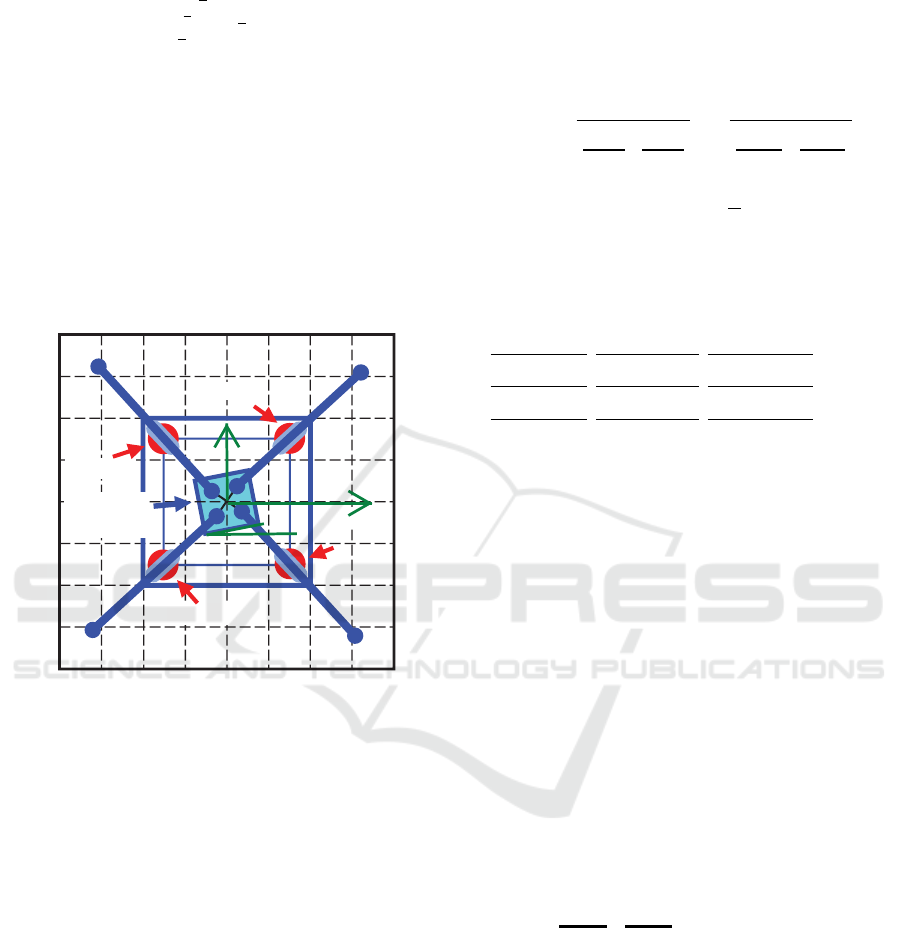
The chosen PKM, the redundant planar parallel robot-
manipulator (Belda, 2010) is characterised by a four-
dimensional input u (four torques) and a three-
dimensional output y (tool center point (TCP) posi-
tions x
TCP
and y
TCP
and rotation angle ϕ
TCP
of robot
movable platform around the vertical axis), see Fig. 1.
drive 1
drive 2
drive 3
drive 4
movable
platform
-0.3 -0.2 -0.1 0 0.1 0.2 0.3 [m]
[m]
0.3
0.2
0.1
0
-0.1
-0.2
-0.3
X
Y
K
Figure 1: Wire frame model of robot.
The dynamics of the robot can be described by
a set of non-linear differential equations representing
equations of motion. They are composed using La-
grange equations (Belda et al., 2007)
¨y = f( ˙y, y) + g(y) u (1)
where y = [ x
TCP
, y
TCP
, ϕ
TCP
]
T
. The corresponding
non-linear continuous-time state-space model is de-
fined as

˙y
¨y

=

˙y
f( ˙y, y)

+

0
g(y)

u
(2)
y =

I 0


y
˙y

.
The nonlinear dynamics in (2) can be transformed
into the linear-like form using a following lineariz-
ing decomposition (linearisation) (Val
´
a
ˇ
sek and Stein-
bauer, 1999)
f( ˙y, y) = a
1
( ˙y, y) ˙y + a
0
( ˙y, y) y =


f
1
( ˙y, y)
f
2
( ˙y, y)
f
3
( ˙y, y)


f( ˙y
r
= 0,y
r
= y
arbitrary
) = 0 (3)
f( ˙y, y) =
f( ˙y, y) − f(0, y)
. ˙y
| {z }
a
1
( ˙y, y)
˙y +
f(0,y) − f(0,y
r
)
.y
| {z }
a
0
( ˙y, y) = 0
y
where dot notation (symbol
∗
.∗
) in denominators
means division element by element. The individual
elements of a
1
( ˙y, y) are defined specifically as fol-
lows:
a
1
( ˙y, y) ˙y =




f
1
( ˙y,y)−f
1
( ˙y
x
,y)
˙x
f
1
( ˙y
x
,y)−f
1
( ˙y
y
,y)
˙y
f
1
( ˙y
y
,y)−f
1
( ˙y
ϕ
,y)
˙
ϕ
f
2
( ˙y,y)−f
2
( ˙y
x
,y)
˙x
f
2
( ˙y
x
,y)−f
2
( ˙y
y
,y)
˙y
f
2
( ˙y
y
,y)−f
2
( ˙y
ϕ
,y)
˙
ϕ
f
3
( ˙y,y)−f
3
( ˙y
x
,y)
˙x
f
3
( ˙y
x
,y)−f
3
( ˙y
y
,y)
˙y
f
3
( ˙y
y
,y)−f
3
( ˙y
ϕ
,y)
˙
ϕ








˙x
˙y
˙
ϕ




(4)
˙y
x
= [0, ˙y,
˙
ϕ]
T
, ˙y
y
= [0, 0,
˙
ϕ]
T
and ˙y
ϕ
= [0, 0, 0]
T
. Note
that a
0
( ˙y, y) = 0 due to properties of the function
f( ˙y, y).
After the decomposition, a linear time-varying
(LTV) state-space model of robot can be written as
follows
˙x = A
c
x + B
c
u (5)
y = C x (6)
where x =

y ˙y

T
, A
c
=

0 I
a
0
( ˙y, y) a
1
( ˙y, y)

,
B
c
=

0
g(y)

, C =

I 0

. Using standard time
discretisation and considering additive bounded dis-
turbances, the following discrete-time linear state-
space model (LSU model) is obtained
x
t
= A
t
x
t−1
+ B
t
u
t−1
| {z }
˜x
t
+ν
t
, ν
t
∼ U
ν
(−ρ,ρ) (7)
y
t
= Cx
t
|{z}
˜y
t
+n
t
, n
t
∼ U
n
(−r, r) (8)
where A
t
= e
A
c
T
s
, B
t
=
t T
s
+T
s
R
t T
s
e
A
c
(t T
s
+T
s
−τ)
B
c
dτ;
˜x
t
and ˜y
t
correspond to the nominal values of x
t
and y
t
;
ν
t
and n
t
are independent and identically distributed
(i.i.d.) state and observation disturbances, they are
uniformly distributed within an orthotope with known
bounds ρ and r, respectively.
Output-feedback MPC for Robotic Systems under Bounded Noise
575

3 BAYESIAN STATE
ESTIMATION OF LSU MODEL
Within the considered Bayesian framework
(K
´
arn
´
y et al., 2005), a controlled system is de-
scribed by:
time evolution model: f (x
t
|
x
t−1
,u
t−1
) (9)
observation model: f (y
t
|
x
t
) (10)
prior pdf: f (x
0
) (11)
Bayesian state estimation (filtering) consists
in the evolution of the posterior pdf f (x
t
|d(t)) where
d(t) is a sequence of observed data records d
t
=
(y
t
,u
t
), d
0
≡ u
0
. The evolution of posterior pdf
f (x
t
|d(t)) is described by a two-steps recursion that
starts from the prior pdf f (x
0
|u
0
) ≡ f (x
0
) (11): (i)
time update that uses theoretical knowledge described
by model (9) and reflects the evolution x
t−1
→ x
t
;
it provides prediction f (x
t
|d(t − 1)), and (ii) data
update that uses theoretical knowledge described by
model (10) and incorporates information about data
d
t
; it provides f (x
t
|d(t)).
The LSU model (7), (8) can be equivalently de-
scribed, using pdf notation (9)–(11), as follows
f (x
t
|u
t−1
,x
t−1
) = U
x
( ˜x
t
− ρ, ˜x
t
+ ρ) (12)
f (y
t
|x
t
) = U
y
( ˜y
t
− r, ˜y
t
+ r) (13)
f (x
0
) = U
x
(x
0
,x
0
) (14)
The exact solution of the Bayesian filtering of
LSU model (12), (13) leads to a very complex form
of posterior pdf. Recently, an approximate Bayesian
state estimation of this model was proposed by one of
authors (Jirsa et al., 2020). It provides the evolution
of the uniformly distributed posterior pdf f (x
t
|d(t))
as follows.
Time Update – The time update starts at t = 1 with
m
0
= x
0
, m
0
= x
0
and it holds
f (x
t
|d(t − 1)) ≈
`
∏
i=1
U
x
t;i
(m
t;i
− ρ
i
,m
t;i
+ ρ
i
) =
= U
x
t
(m
t
− ρ, m
t
+ ρ), (15)
where m
t
= [m
t;1
,..., m
t;`
]
0
, m
t
= [m
t;1
,..., m
t;`
]
0
, ` is
the size of x,
m
t;i
=
`
∑
j=1
min(A
i j
x
t−1; j
+ B
i
u
t−1
,A
i j
x
t−1; j
+ B
i
u
t−1
),
(16)
m
t;i
=
`
∑
j=1
max(A
i j
x
t−1; j
+ B
i
u
t−1
,A
i j
x
t−1; j
+ B
i
u
t−1
).
Data Update – In data update step, the observation
y
t
(13) is processed as y
t
− r ≤ Cx
t
≤ y
t
+ r by the
Bayes rule together with the prior (15) from the time
update. The resulting uniform pdf posses a support in
the form of polytope. It is approximated by a uniform
pdf with an orthotopic support
f (x
t
|d(t)) ≈ U
x
t
(x
t
, x
t
). (17)
The proposed approximation is based on a minimis-
ing of Kullback-Leibler divergence of two pdfs (Jirsa
et al., 2020).
The result of the approximate Bayesian filtering
(17) says that the state estimate ˆx
t
lies within a set
ˆx
t
∈ hx
t
,x
t
i (18)
where all points have the same probability. In the
previous paper of authors (Kukli
ˇ
sov
´
a Pavelkov
´
a and
Belda, 2019), the point state estimate for control al-
gorithm was chosen to correspond to the centre of the
orthotope in (17)
ˆx
t
=
x
t
+ x
t
2
. (19)
Here, we integrate the choice of point estimate into
the optimisation step of control design.
4 CONTROL DESIGN
This section introduces two algorithms of output-
feedback MPC, namely the positional and the incre-
mental algorithm. To design an optimal control ac-
tion, MPC employs predictions of expected future
outputs of controlled system represented by a state
space model. The main design elements, i.e. equa-
tions of predictions and relevant quadratic cost func-
tion are introduced in the following subsections.
4.1 Predictions of Future Outputs
The equations of predictions express the relationship
between future predicted outputs and unknown con-
trol actions. They are composed using current state
estimate in nominal parts of model (7) and (8). For
simplicity, we omit here the time indices, i.e., A
t
→ A
and B
t
→ B, as for one optimisation step, the matrices
are constant for whole prediction horizon N.
Prediction equations for the positional control al-
gorithm (Kukli
ˇ
sov
´
a Pavelkov
´
a and Belda, 2019) are
composed as follows
ˆ
Y
t+1
=

ˆy
T
t+1
, · · · , ˆy
T
t+N

T
= F
1
ˆx
t
+ G
1
U
t
,
U
t
=

u
T
t
, · · · , u
T
t+N−1

T
(20)
ICINCO 2021 - 18th International Conference on Informatics in Control, Automation and Robotics
576

where
F
1
=





CA
.
.
.
CA
N−1
CA
N





, G
1
=





CB 0 ··· 0
.
.
.
.
.
.
.
.
.
.
.
.
CA
N−2
B ··· CB 0
CA
N−1
B ··· CAB CB





.
To achieve integral property in the design, the
nominal parts of model (7) and (8) are rewritten in
incremental forms as follows
∆ ˆx
t+1
= ˆx
t+1
− ˆx
t
= A ∆ ˆx
t
+ B ∆u
t
∆ ˆy
t+1
= ˆy
t+1
− y
t
= C ∆ ˆx
t+1
.
(21)
The prediction equations for incremental control
algorithm are composed recursively using the model
(21). The recursivity is involved by the index j =
1, · · · , N that determines individual discrete time in-
stants for the horizon N,
∆ ˆx
t+ j
= A
j
∆ ˆx
t
+
j
∑
i=1
A
i−1
B∆u
t+ j−i
(22)
∆ ˆy
t+ j
= CA
j
∆ ˆx
t
+
j
∑
i=1
CA
i−1
B∆u
t+ j−i
(23)
The evolution of the full-value predictions
of the system outputs ˆy is
ˆy
t+ j
= y
t
+
j
∑
i=1
∆ ˆy
t+i
(24)
The relevant matrix notation of (24) is as follows
ˆ
Y
t+1
= F
I
y
t
+ F
2
∆ ˆx
t
+ G
2
∆U
t
(25)
where
ˆ
Y
t+1
= [
ˆy
T
t+1
··· ˆy
T
t+N
]
T
,F
I
= [
I · · · I
]
T
,
F
2
=





CA
.
.
.
N
∑
i=1
CA
i





, G
2
=





CB ··· 0
.
.
.
.
.
.
.
.
.
N
∑
i=1
CA
i−1
B ··· CB





4.2 Cost Function
The behaviour of a control process is influenced by
the choice of the cost function. We use a quadratic
cost function. It balances control errors, i.e. differ-
ences between predicted outputs and reference values,
against amount of input energy given by control vec-
tor or control increments, respectively.
The cost function for the positional algorithm
(Kukli
ˇ
sov
´
a Pavelkov
´
a and Belda, 2019) is
J
t
=
N
∑
j=1

kQ
yw
( ˆy
t+ j
− w
t+ j
)k
2
2
+ kQ
u
u
t+ j−1
k
2
2

(26)
The cost function for the incremental algorithm is
J
t
=
N
∑
j=1
n
k(Q
yw
( ˆy
t+ j
− w
t+ j
)k
2
2
+


Q
∆u
∆u
t+ j−1


2
2
o
(27)
where k.k
2
2
means the squared Euclidean norm.
4.3 Minimization Procedure
Optimality criterion is defined as follows
min
U
t
J
t
(
ˆ
Y
t+1
,W
t+1
,U
t
), U
t
∈ {U
t
,∆U
t
} (28)
s.t. state space model (7) and (8)
set state estimate ˆx
t
(18)
where
ˆ
Y
t+1
are prediction equations (20) or (25), re-
spectively, W
t+1
represents a sequence of references
W
t+1
=

w
T
t+1
, · · · , w
T
t+N

T
(29)
The involved cost function J
t
(26) or (27) are
rewritten into the square-root form
J
t
= J
T
t
J
t
(30)
Positional Algorithm
The square-root J
t
of the cost function J
t
(30) is
J
t
=

Q
YW
0
0 Q
U

ˆ
Y
t+1
−W
t+1
U
t

=

Q
YW
F ˆx
t
+ Q
YW
GU
t
− Q
YW
W
t+1
Q
U
U
t

. (31)
where Q
YW
, Q
∆U
and Q
U
are penalisation matrices
defined as follows
Q
T

Q

=



Q
T
∗
Q
∗
0
.
.
.
0 Q
T
∗
Q
∗









subscripts , ∗ :
 ∈ {YW, ∆U, U }
∗ ∈ {yw, ∆u, u}
(32)
Considering minimization of the square-root J
t
as a specific solution of least-squares problem leads
to the following algebraic equation (Kukli
ˇ
sov
´
a Pa-
velkov
´
a and Belda, 2019):

Q
YW
G Q
YW
(W
t+1
− F ˆx
t
)
Q
U
0

U
t
−I

= 0
(33)
Output-feedback MPC for Robotic Systems under Bounded Noise
577

Incremental Algorithm
The square-root J
t
of the cost function J
t
(30) is
J
t
=

Q
YW
0
0 Q
∆U

ˆ
Y
t+1
−W
t+1
∆U
t

=

Q
YW
(F
I
y
t
+ F
2
∆x
t
+ G
2
∆U
t
− W
t+1
)
Q
∆U
∆U
t

. (34)
Considering minimization of the square-root J
t
as
a specific solution of least-squares problem leads to
the following algebraic equation:

Q
YW
G
2
Q
YW
Z
Q
∆U
0

∆U
t
−I

= 0
(35)
with Z = W
t+1
− F
I
y
t
− F
2
∆x
t
.
———————————————–
The over-determined system (33) or (35), respec-
tively, can be rewritten into the condensed general
form A U
t
= b.
This form can be transformed by orthogonal-
triangular decomposition (Lawson and Hanson, 1995)
into the following form and solved for unknown U
t
Q
T
A U
t
= Q
T
b assuming that A = QR
R
1
U
t
= c
1
(36)
where U
t
∈ {U
t
,∆U
t
}, Q
T
is an orthogonal matrix
that transforms matrix A into upper triangle R
1
.
It is indicated by the following equation diagram
A U
t
=
b
⇒
@
@
@
@
R
1
0
U
t
=
c
1
c
z
(37)
Vector c
z
represents a loss vector. Euclidean norm
kc
z
||
2
corresponds to the square-root of the minimum
of cost function (26) or (27), i.e., J
t
= c
T
z
c
z
.
In the previous paper of authors (Kukli
ˇ
sov
´
a Pa-
velkov
´
a and Belda, 2019), the transformation into
(36) was performed once using the point state esti-
mate (19).
Here, we consider the set estimate (18). The
transformation into (36) is performed successively for
properly selected points from the whole set. Sub-
sequently, the realisation with the minimal value of
kc
z
||
2
is chosen as the result.
For control, only the first elements corresponding
to u
t
are used from computed vector U
t
. Then, for the
positional algorithm
u
t
= MU
t
(38)
and for the incremental algorithm
u
t
= u
t−1
+ M ∆U
t
(39)
where matrix M is defined as M = [I
n
u
, 0
n
u
, ··· , 0
n
u
],
n
u
is dimension of vector of control actions u
t
.
Algorithmic Summary
The following summary describes a sequence per-
formed during the control process.
Initialisation:
i. set the initial state ˆx
0
∈ hx
0
,x
0
i and control u
0
ii. set t := 1, t ≥ 1
iii. load the reference trajectory w
1
, w
2
, ..., w
t
iv. initialise nonlinear continuous model (1)
v. set r and ρ for LSU model (7) and (8)
vi. set N, Q
∗
in (26) or (27), respectively
On-line phase:
1. update the model matrices A
t
, B
t
in (7) and (8)
2. select representative points from the set (18)
3. compute c
z
(37) for selected points
4. choose the control input u
t
(38) or (39) that cor-
responds to minimal kc
z
k
2
5. simulate a new state of model (1) in t + 1
6. set time t := t +1
7. measure disturbed system output y
t
8. obtain the set state estimate ˆx
t
∈ hx
t
,x
t
i (18)
9. if t < t, go to 1.
End, result evaluation.
5 EXPERIMENTS
This section demonstrates the proposed output-
feedback MPC applied to the motion control of PKM
robot depicted in Figure 1 represented by the model of
the machine dynamics. It is described in Sec. ’Robot
model’, specifically by the equations (1)-(8).
5.1 Experiment Setup
The real controlled system, as depicted in Figure 2
on the left, is simulated by (1) with an added uni-
form noise. The testing trajectory is depicted in Fig-
ure 2 on the right.
ICINCO 2021 - 18th International Conference on Informatics in Control, Automation and Robotics
578

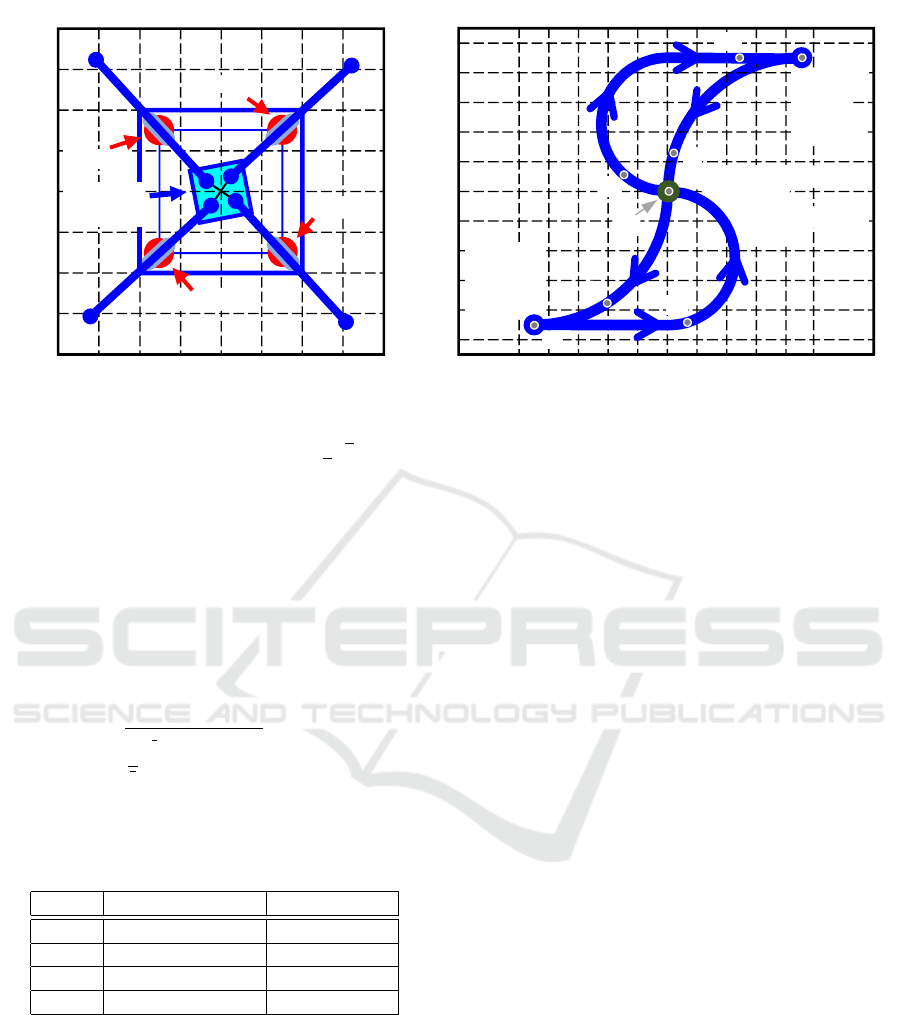
drive 1
drive 2
drive 3
drive 4
movable
platform
-0.3 -0.2 -0.1 0 0.1 0.2 0.3 [m]
[m]
0.3
0.2
0.1
0
-0.1
-0.2
-0.3
[m]
0.04
0.02
0
-0.02
-0.04
-0.04 -0.02 0 0.02 0.04 [m]
turning
point
v
t
= 0
turning
point
v
t
= 0
initial, final points
v
t
= 0
running point
v
t
 0
1s
2s
3s
4s
5s
6s
7s
0s
Figure 2: Considered robot ’Moving Slide’ and used testing trajectory.
The state estimates ˆx
t
∈ hx
t
,x
t
i (18)
are obtained using the model (7) and (8)
with the noise bounds set as follows:
ρ = 10
−6
[m,m,rad, m s
−1
,ms
−1
,rad s
−1
]
T
,
r = 10
−3
[m,m,rad]
T
. The control parameters in
(26) or (27) are set as follows: N = 10; Q
yw
= I,
Q
u
= 10
−2
I, Q
∆u
= 2.5 ·10
−5
I, where I is the identity
matrix of the appropriate order.
The quality of the control process is evaluated by
the visual comparison of the results and by the root
mean square error (RMSE) between outputs y
t
and
references w
t
RMSE
i
=
v
u
u
t
1
t
t
∑
t=1
(y
t;i
− w
t;i
)
2
, i = {1, 2, 3}. (40)
The following experiments were performed for
the robot motion along the reference trajectory as de-
picted in Figure 2:
control algorithm state estimate
Exp.1 positional (38) point (19)
Exp.2 positional (38) set (18)
Exp.3 incremental (39) point (19)
Exp.4 incremental (39) set (18)
5.2 Results and Discussion
The results of individual experiments are shown in
Figures 3 – 8. Figure 3 and Figure 4 show time histo-
ries for the positional algorithm. The positional algo-
rithm with set state estimate (Exp. 2) reaches smaller
dispersion control errors. Control errors do not tend
to zero since both experiments Exp. 1 and Exp. 2
were realized with positional algorithm that has pro-
portional character only. It is useful for fast repeated
manipulation motion that does not need track the ref-
erence trajectory or stay in one position precisely but
with smaller dynamic demands on robot drives.
Figure 5 shows the values kc
z
||
2
in (37) for the po-
sitional algorithm (38) and the state estimate set (18)
in the selected times, namely 1s, 2s, 3s, 4s, 5s and 6s.
Filled blue circle indicates the searched cost function
minimum that is used for the control design in accord
with (37).
Figure 6 and Figure 7 show time histories for the
incremental algorithm. The incremental algorithm
with set state estimate (Exp. 4) reaches smaller disper-
sion control errors again. Control errors do not tend
to zero, but they are symmetrically distributed around
horizontal axis x since both experiments Exp. 1 and
Exp. 2 were realized with incremental algorithm that
push controlled system towards zero. However, due
to noise, it is asymptotic trend.
Figure 8 shows the values kc
z
||
2
in (37) for the
incremental algorithm (39) and the state estimate set
(18) in the selected times, namely 1s, 2s, 3s, 4s, 5s
and 6s. Filled blue circle indicates the searched cost
function minimum that is used for the control design
in accord with (37).
The numerical comparison of RMSE
i
values for
experiments Exp.1– Exp.4 is presented in Table 1.
The results are comparable. However, the optimisa-
tion in Exp. 2 and Exp. 4 takes into account cost val-
ues that balance not only control error but also mag-
nitudes of control actions or their increments.
6 CONCLUSION
The paper proposes a novel solution to the output-
feedback MPC under bounded state and output dis-
Output-feedback MPC for Robotic Systems under Bounded Noise
579

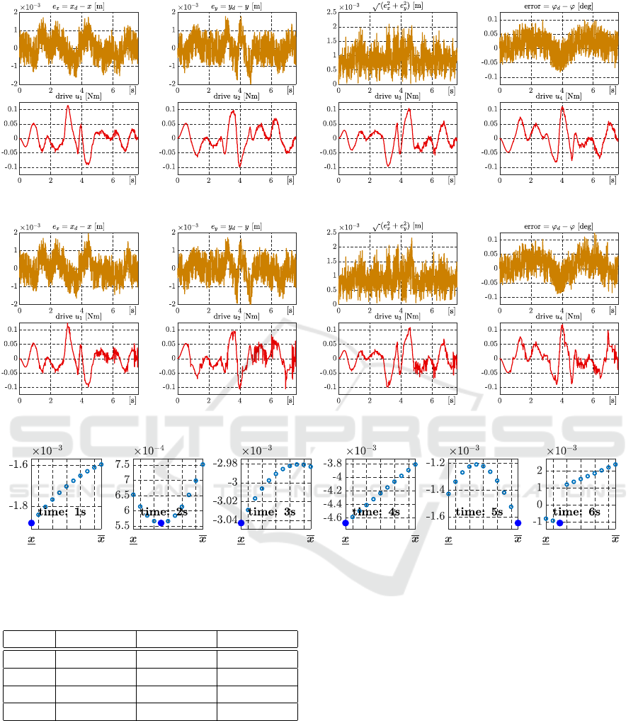
Figure 3: Time histories of control errors and control actions (Exp. 1).
Figure 4: Time histories of control errors and control actions (Exp. 2).
||c
z
||
2
Figure 5: Selected time instants with the cost function for the set state estim. (Exp. 2).
Table 1: RMSE
i
(40) for the individual experiments Exp.1–
Exp.4.
RMSE
1
RMSE
2
RMSE
3
Exp.1 0.694·10
−3
0.705·10
−3
0.705·10
−3
Exp.2 0.694·10
−3
0.721·10
−3
0.731·10
−3
Exp.3 0.622·10
−3
0.633·10
−3
0.669·10
−3
Exp.4 0.626·10
−3
0.644·10
−3
0.678·10
−3
turbances. Comparing to the previous work of author
(Kukli
ˇ
sov
´
a Pavelkov
´
a and Belda, 2019), the proposed
algorithm enables further reduction of the involved
cost function (28) by considering set state estimates
(18) and their inclusion into the minimization step.
The selection of a suitable points from (18) is made
by the user.
The proposed solution considers an unconstrained
positional and incremental MPC. The overshoot of
possible constraints is prevented by the appropriate
design of reference trajectory and its suitable time
parametrisation (Belda and Novotn
´
y, 2012).
The presented research is important for mechan-
ical systems where bounded noises are present fre-
quently but usually modelled by unbounded Gaussian
distribution. In practice, the use of unbounded noises
leads to over-conservative design, which induces a re-
markable increase in the costs. The stochastic mod-
els built on bounded noises prevent these problems
(d’Onofrio, 2013).
Next research will try to formulate the optimal se-
lection of the points from the set (18). Also, a more
flexible sets of estimates will be considered, namely
zonotopes (Combastel, 2015), that will provide the
less conservative guaranteed estimates comparing to
the currently used orthotopic set.
ICINCO 2021 - 18th International Conference on Informatics in Control, Automation and Robotics
580

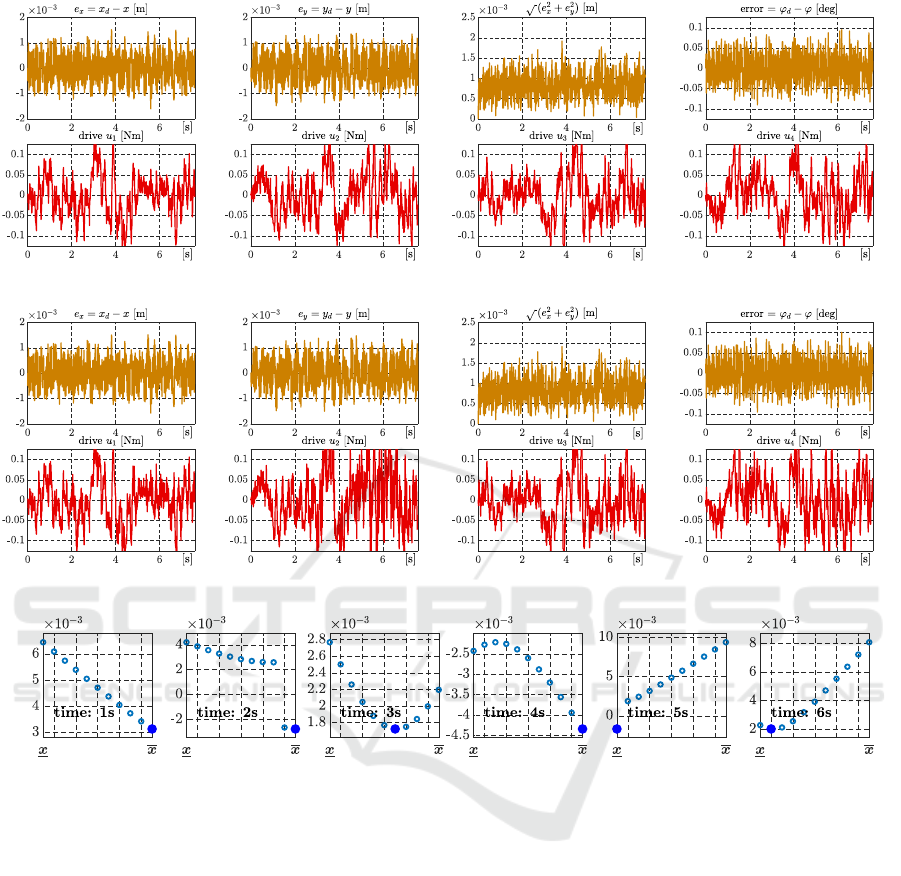
Figure 6: Time histories of control errors and control actions (Exp. 3).
Figure 7: Time histories of control errors and control actions (Exp. 4).
||c
z
||
2
Figure 8: Several time instants with the cost function for the set state estim. (Exp. 4).
REFERENCES
Belda, K. (2010). Robotic device, Ct. 301781 CZ, Ind. Prop.
Office.
Belda, K., B
¨
ohm, J., and P
´
ı
ˇ
sa, P. (2007). Concepts of
model-based control and trajectory planning for paral-
lel robots. In Klaus, S., editor, Proc. of 13th IASTED
Int. Conf. on Robotics and Applications, pages 15–20.
Acta Press.
Belda, K. and Novotn
´
y, P. (2012). Path simulator for ma-
chine tools and robots. In Proc. of the 17th Int. Conf.
on Methods and Models in Automation and Robotics,
pages 373–378.
Brunner, F. D., M
¨
uller, M. A., and Allg
¨
ower, F. (2018). En-
hancing output-feedback mpc with set-valued moving
horizon estimation. IEEE Transactions on Automatic
Control, 63(9):2976–2986.
Combastel, C. (2015). Zonotopes and kalman observers:
Gain optimality under distinct uncertainty paradigms
and robust convergence. Automatica, 55:265–273.
d’Onofrio, A. (2013). Bounded Noises in Physics, Biology,
and Engineering. Springer.
Jirsa, L., Kukli
ˇ
sov
´
a Pavelkov
´
a, L., and Quinn, A. (2020).
Approximate Bayesian prediction using state space
model with uniform noise. In Informatics in Con-
trol Automation and Robotics, volume 613 of LNEE,
pages 552–568. Springer.
K
´
arn
´
y et al. (2005). Optimized Bayesian Dynamic Advising:
Theory and Algorithms. Springer.
Khlebnikov, M. V., Polyak, B. T., and Kuntsevich, V. M.
(2011). Optimization of linear systems subject to
bounded exogenous disturbances: The invariant el-
lipsoid technique. Automation and Remote Control,
72(11):2227–2275.
K
¨
ogel, M. and Findeisen, R. (2017). Robust output feed-
back MPC for uncertain linear systems with reduced
Output-feedback MPC for Robotic Systems under Bounded Noise
581

conservatism. IFAC-PapersOnLine, 50(1):10685 –
10690.
Kukli
ˇ
sov
´
a Pavelkov
´
a, L. and Belda, K. (2019). Output-
feedback model predictive control for systems under
uniform disturbances. In 2020 7th International Con-
ference on Control, Decision and Information Tech-
nologies (CoDIT), pages 897–902.
Lawson, C. and Hanson, R. (1995). Solving least squares
problems. Siam.
Luces, M., Mills, J. K., and Benhabib, B. (2017). A Review
of Redundant Parallel Kinematic Mechanisms. Jour-
nal of int. & robot. systems, 86(2):175–198.
Mammarella, M. and Capello, E. (2020). Tube-Based
Robust MPC Processor-in-the-Loop Validation for
Fixed-Wing UAVs. Journal of int. & robot. systems,
100(1):239–258.
Qiu, Q., Yang, F., Zhu, Y., and Mousavinejad, E. (2020).
Output feedback model predictive control based on
set-membership state estimation. IET Control Theory
Applications, 14(4):558–567.
Val
´
a
ˇ
sek, M. and Steinbauer, P. (1999). Nonlinear control
of multibody systems. In Proc. of Euromech, pages
437–444.
Zenere, A. and Zorzi, M. (2017). Model Predictive Control
meets robust Kalman filtering. IFAC-PapersOnLine,
50(1):3774–3779.
ICINCO 2021 - 18th International Conference on Informatics in Control, Automation and Robotics
582