Deep Generative Models to Extend Active Directory Graphs with

Honeypot Users

Ond

rej Luk

and Sebastian Garcia

Faculty of Electrical Engineering, Czech Technical University, Prague, Czech Republic

Keywords:

Generative Models, Autoencoders, Active Directory, Honeypots, Deep Learning.

Abstract:

Active Directory (AD) is a crucial element of large organizations, given its central role in managing access

to resources. Since AD is used by all users in the organization, it is hard to detect attackers. We propose to

generate and place fake users (honeyusers) in AD structures to help detect attacks. However, not any honeyuser

will attract attackers. Our method generates honeyusers with a Variational Autoencoder that enriches the AD

structure with well-positioned honeyusers. It ﬁrst learns the embeddings of the original nodes and edges in the

AD, then it uses a modiﬁed Bidirectional DAG-RNN to encode the parameters of the probability distribution

of the latent space of node representations. Finally, it samples nodes from this distribution and uses an MLP

to decide where the nodes are connected. The model was evaluated by the similarity of the generated AD with

the original, by the positions of the new nodes, by the similarity with GraphRNN and ﬁnally by making real

intruders attack the generated AD structure to see if they select the honeyusers. Results show that our machine

learning model is good enough to generate well-placed honeyusers for existing AD structures so that intruders

are lured into them.

1 INTRODUCTION

From the range of attacks that organizations face,

those to the internal network are the most critical.

Companies such as Sony, Austria Telekom, NTT,

and Citrix have been compromised in their internal

networks (Zetter, 2014; Cimpanu, 2020b; Cimpanu,

2020a; Whittacker, 2019). These attacks are usually

to their Active Directory (AD) to gain access to in-

ternal resources (Crabtree, 2020). AD stores sensitive

data, and since it is used by all internal users, it is

difﬁcult to detect attacks in the AD by differentiting

between normal and attacker behaviors.

There are three common defenses in AD. First,

to stop attackers from accessing the AD by using

network segmentation, by limiting access (Metcalf,

2015), by hardening AD conﬁgurations, or by moni-

toring system events (Nurfauzi, 2020; Metcalf, 2015).

Second, to detect anomalies in the use of AD(Karlin

et al., 2018). Third, to use honeyusers.

A honeyuser is a fake user disguised as a real user

and designed to attract attackers (de Barros, 2003).

Since users should not interact with honeyusers, any

interaction triggers a detection. Honeyusers have

https://orcid.org/0000-0002-7922-8301

https://orcid.org/0000-0001-6238-9910

been used for fake bank accounts and database, but

rarely in AD. To maximize the chance of being at-

tacked, the correct placement of the honeyuser in the

AD is essential.

We propose a deep learning variational autoen-

coder model which generates both features and place-

ment location of honeyusers in AD graphs. First, a

graph representation of an existing AD is extracted.

Second, the graph is encoded using a Bidirectional

Directed Acyclic Graph Recurrent Neural Network

(DAG-RNN). The latent space of the encoded graphs

is represented by a multivariate Normal didstribution.

Third, new nodes are sampled from the probability

distribution and a Multilayer Perceptron (MLP) is

used to predict their position in the extended graph.

The model outputs a set of nodes to add to the AD,

their features and where (to which nodes) they should

be connected.

Since AD data is difﬁcult to obtain, we gener-

ated syntetic graphs by boosting them with a small

sample of real AD structures. These syntetic datasets

were used to train and evaluate our model against the

GraphRNN technique (You et al., 2018). We also

evaluated the quality of the honeyusers by publishing

a game to attack a real AD on the Internet. This game

helped understand if real attackers are more lured into

140

Lukáš, O. and Garcia, S.

Deep Generative Models to Extend Active Directory Graphs with Honeypot Users.

DOI: 10.5220/0010556601400147

In Proceedings of the 2nd International Conference on Deep Learning Theory and Applications (DeLTA 2021), pages 140-147

ISBN: 978-989-758-526-5

the honeyusers placed by our model.

Results show that the DAG-RNN model can gen-

erate new honeyuser-enriched AD graphs that are in

average 80% similar to the original graph. It can

also place honeyusers in organic positions 94% of

the time. Preliminary results from the real-life game

are inconclusive but suggest an attackers’ tendency to

prefer the DAG-RNN generated honeyusers.

The contributions of this paper are:

• A DAG-RRN autoencoder for extending AD

graphs with honeyusers.

• The ﬁrst Bidirectional DAG-RNN models applied

to the domain of honeyusers generation.

• An evaluation with real-life attackers.

• A public implementation of the DAG-RNN model

that only depends on Tensorﬂow 2.

• A sythetic dateset of AD graphs.

The rest of the paper is organized as follows: Sec-

tion 2 describes the related work; Section 3 describes

the generation of the dataset; Section 4 describes the

deep learning method; Section 5 describes the evalu-

ations of the model; Section 6 shows the results; and

Section 7 makes the conclusion.

2 RELATED WORK

Active Directory (AD) has been analyzed as a target

due to its importance inside companies (Case, 2016),

with the most common detection approach being to

search the AD logs for anomalies (Matsuda et al.,

2018).

Common protecting AD solutions include hard-

ening and monitoring tools (Grimes, 2006), with the

main tool for detecting malicious activities being the

Advanced Threat Analytics by Microsoft (Microsoft,

2015), which detects abnormal activity. Some tools

manage fake accounts (Berg, 2019), but do not gen-

erate new honeyusers. The DCEPT tool (Bettke and

Stewart, 2016) creates fake accounts in memory of

end-points. To our knowledge, there is no research

to automatically generate honeypots in AD (Valicek

et al., 2017).

In other areas, automation and machine learning

methods were used to design honeypots. Techniques

include state machines to generate scripts (Leita et al.,

2005) for the honeypot honeyd (Provos, 2003). Rein-

forcement Learning has also been used for generating

honeypot responses to extend the duration of the at-

tack (Dowling et al., 2018). Game Theory was also

used to place honeypots as a two-player interaction

game (Tian et al., 2019).

Graph Neural Networks (GNN) were used for de-

tection, generation, and classiﬁcation of graphs. A

prominent work is GraphRNN (You et al., 2018),

where the graph is iteratively created using two re-

current modules, one for nodes and one for graphs.

GraphRNN outperforms Graph convolutional neural

networks on the generation of undirected graphs.

Graph Variational Autoencoders were used to gen-

erate small undirected graphs in molecule modelling

with success (Simonovsky and Komodakis, 2018).

The method, however, lacks good scaling and prede-

ﬁnes the maximal size of structures.

Graph Recurrent Attention Networks (Liao et al.,

2019), showed success in modeling protein data, ex-

ceeding both GrapVAE and GraphRNN. The tech-

nique combined recurrent GNN with attention layers.

Directed Acyclic Graphs (DAG) were used with

custom RNN cells to analyze a DAG structure and

produce simpliﬁcations of formulas (Kaluza et al.,

2018). A DAG-to-DAG also learnt the satisﬁability

of formulas in propositional logic (Amizadeh et al.,

2019). Both works used the Encoder-Decoder archi-

tecture on top of graph recurrent cells. As far as we

know, there are no publications using generative mod-

els for honeypot generation.

3 ARTIFICIAL DATASET

Production AD environments have sensitive Person-

ally Identiﬁable Information (PII) from users, therfore

it is hard to obtain good datasets of real AD structures.

We solved the issue by obtaining few real AD

structures by signing Non-disclosure Agreements

(NDAs) and using these samples for boosting the gen-

eration of artiﬁcial datasets. These datasets maintain

the same characteristics of the real AD, with the help

and veriﬁcation of security experts.

We created four artiﬁcial datasets which differ in

the number of nodes and edges. Each one contains a

large number of graphs with similar number of nodes.

All graphs are valid Directed Acyclic Graphs that fol-

low the restrictions of the real AD, such as which

groups have more users.

3.1 Extracting Active Directory Data

The structure of real AD has to be extracted to be used

in our model. We used the tool Sharphound (Vazarkar,

2016) for this.

We ﬁlter the real ADs to only retain ﬁve node

types and their edges. The types used in our datasets

are: User, Computer, Domain, OrganizationalUnit

Deep Generative Models to Extend Active Directory Graphs with Honeypot Users

141

(OU), and Group. The number of edges for the indi-

vidual graphs is sampled from a Gaussian distribution

using parameters estimated from real AD structures.

To generate our four artiﬁcial datasets, we then

used the random DAG generation of the NetworkX

library (Hagberg et al., 2008). All generated graphs

in each dataset have the same node-to-edge ratio and

node type as the real AD structures. Table 1 shows

the properties of the datasets. The main difference

between them is their size.

Table 1: Artiﬁcial datasets with number of graphs, num-

ber of nodes, mean amount of vertices and mean amount of

edges.

Dataset graph

size

# sam-

ples

Mean

|V |

Mean

|E|

AD15 15 2,000 12.51 19.02

AD50 50 2,000 39.88 65.49

AD150 150 2,500 115.11 192.49

AD500 500 1,000 353.36 600.17

We assume that the number of edges to other

nodes is an important criterion that inﬂuences why an

attacker chooses that user. Therefore, the usefulness

of a honeyuser node for being a good target is related

to how many connections it has and to which nodes.

Each of the artiﬁcial datasets was splitted for train-

ing and validation (4/5), and testing (1/5). The test-

ing was not used until the ﬁnal evaluation. The train-

ing/validation sets were shufﬂed.

4 GRAPH GENERATION

FRAMEWORK

Our framework starts by creating a graph representa-

tion from the AD structure. Then, the graph is en-

coded into a latent space using the node type em-

beddings and our bi-directional DAG-RNN encoder.

From the encoder, new nodes are sampled and used as

input for the decoder, which predicts their placement.

Lastly, we generate attributes of the new nodes before

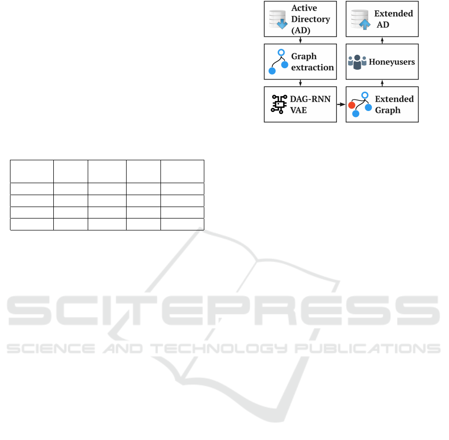
inserting them back into the AD. Figure 1 shows a

diagram of the framework.

4.1 From AD to Graph Representation

The ﬁrst step is representing the AD as a directed

acyclic graph(DAG). Only six basic node types re-

lated to users are present in the graph (Section 3). The

acyclicity allows for topological sorting of the nodes

in the DAG, which is essential for the encoding pro-

cess. Each graph is represented by A, and adjacency

Figure 1: Diagram of our framework. First, from an AD to

graph. Second, embedding of nodes. Third, process nodes

with a DAG-RNN Variational Autoencoder. Fourth, pre-

dicts locations of nodes. Fifth, enrich the features of nodes.

Sixth, inserts the nodes as honeyusers in the AD.

node matrix, A

its transposed version for reverse

directionality, and a matrix X that represents one-

hot encoded node features. These matrices are zero

padded to align the shapes in the mini-batch during

the training. The padded nodes are masked during the

whole training. The matrix X is input to an embed-

ding layer that outputs the matrix X

with the embed-

dings that represent similarities between the nodes.

4.2 DAG-RNN Variational

AutoEncoder

The node embeddings and structural information in A

and A

are used in the autoencoding process (Kingma

and Welling, 2014). The topology-aware, RNN-based

Variational Autoencoder (DAG-RNN VAE) shown in

Figure 2 learns latent space representation of each

node in the graph and can generate new nodes with

similar properties.

The DAG-RNN VAE inputs matrices X

, A and

and outputs matrix

A, which contains the place-

ments of the proposed nodes. A multi-variate Gaus-

sian parametrizes the latent space z in which the En-

coder represents the original nodes. Such architecture

allows sampling of the latent space representation of

new nodes. The MLP Decoder predicts the probabil-

ity of the presence of an edge between a pair of nodes.

During the training phase, the model attempts to re-

construct the original adjacency matrix. During gen-

eration, edges from the original nodes to newly sam-

pled are predicted.

4.2.1 DAG-RNN Encoder

The DAG-RNN layer contains bi-directional Gated

Recurrent Units (GRUs), which process the nodes se-

quentially following the ordering given by A and A

Unlike a traditional GRU, the output of a DAG-RNN

DeLTA 2021 - 2nd International Conference on Deep Learning Theory and Applications

142

Figure 2: Overview of the VAE. Inputs are, matrix X (one-

hot encoded node types), adjacency matrix A, and its trans-

pose A

. Rows follow a topological ordering. The VAE

consists of an Encoder (Embedding layer and DAG-RNN

layer) which projects the inputs in a latent space z, and a

Decoder (MLP) which reconstructs the adjacency matrix

is not fed back as recurrent input, but stored in the ma-

trix

−→

H (

←−

H for the unit processing the reversed graph).

In a directed graph there can be multiple previ-

ous states (a node can have numerous direct predeces-

sors). Let G = hV

, E

i be a graph used as input for

our method, with V

the set of vertices of G and E

the set of edges. By topologically ordering the nodes

of G it is guaranteed that ∀v

⊆ V

, all of its predeces-

sors have been already been processed in timestamps

t < i and their latent space representation is stored in

−→

H .

When computing the previous state for node v

we use the corresponding slice of matrix A to create a

mask for

−→

H . With the mask, we can combine the hid-

den states using summation which results in the pre-

vious state for the GRU. Similarly with the reversed

graph, we use A

for masking

←−

H .

The aggregation of hidden states forces the nodes

to be connected in a similar way as nodes in the AD.

This makes it possible to generate honeyusers that

will be part of the most populated groups.

As a last step, we sum the directional results in

−→

and

←−

H using to obtain a single output matrix H.

Apart from matrix H, which contains the latent

space representation of all nodes in the graph, the

Encoder outputs vectors µ and σ - the parameters of

a multivariate Normal distribution which regularizes

the latent space. Each of the parameters is estimated

by a single MLP. These parameters are used for (i) la-

tent loss computation, (ii) sampling of the new nodes

to be added in the graph.

4.2.2 Decoder

The decoder samples one node from the probability

distribution for each pre-required honeyuser. The ma-

trix of all requested nodes is Z. Then, it pairs the sam-

pled new nodes with the existing nodes doing a Carte-

sian product between Z and H. Each pair is input to

Figure 3: Bi-directional DAG-RNN layer. The inputs to

the GRU cell are the embeddings of the node X

and the

aggregation of previous states following the topology of the

graph. Matrices A and A

are used to mask the previous

states stored in

−→

H and

←−

H . The outputs of both directions

are combined using sum.

an MLP that estimates if the pair should be kept, stor-

ing this estimation in

A. The sigmoid activation of the

MLP has a threshold value of 0.2.

4.2.3 Loss Functions

Since the model is trained all at once, we used a com-

pound weighted loss that is the sum of two functions:

a reconstruction loss and a latent loss.

The Reconstruction Loss estimates the auto

encoder information loss using the Sigmoid Focal

Loss(Lin et al., 2017) (Equation (1), which is a mod-

iﬁcation of the binary cross-entropy loss for highly

imbalanced classes. In our model, the presence or ab-

sence of an edge in

A is treated as a binary classiﬁca-

tion.

FL(p

) = −α

(1 − p

)

log(p

) (1)

FL is a modiﬁcation of binary cross-entropy us-

ing the parameters α and γ to address the imbalance

and the different difﬁculty of classifying classes. The

γ parameter scales the classiﬁcation difﬁculty of the

minority class. In FL, (1 − p

)

is a modulating fac-

tor, while pt is a notational convenience deﬁned as

= p if y = 1 and p

= (1 − p) otherwise. Where y

speciﬁes the ground-truth class, p is the prediction.

The Latent Loss estimates the difference between

the distribution of the latent space and the Normal

distribution. We used the Kullback-Leibler Diver-

gence (Joyce, 2011) (Equation 2). D

measures the

distance between the latent distribution Q and another

distribution (Normal for us) as the prior P.

(PkQ) =

∑

x∈X

P(x)log(

P(x)

Q(x)

) (2)

Deep Generative Models to Extend Active Directory Graphs with Honeypot Users

143

Where X is the probability space, and P = N(0, 1).

The loss function is a weighted sum of the Focal

loss and the Latent loss, shown in Equation 3.

L =





+ |z|D



, z



kN (0, 1)



(3)

Where n is the number of nodes, A is the adja-

cency matrix,

A is the estimated adjacency matrix,

and z

are the estimated parameters of the nor-

mal distribution. The Focal Loss is divided by two

since we only estimate half of

A, that is a lower trian-

gular matrix.

4.3 Honeyuser Attributes Generation

For each newly generated node, we still need to gen-

erate its AD attributes before adding them to the ﬁ-

nal graph. For the attributes dependent of the posi-

tions, such as Distinguished Name (DN), it is neces-

sary to build it based on the position path. For the

attributes that are independent of the position, they

are randomly generated using external tools such as

Faker (Faraglia, 2012). We verify that the properties

of an AD are not violated.

Once the attributes were generated, we insert the

extended AD graph back into the original AD server

using Powershell cmdlets or LDAP addition queries.

4.4 Implementation and Complexity

The DAG-RNN framework was implemented based

on Tensorﬂow 2 and Keras so it can be used in CUDA

GPUs. As far as we know, it is the ﬁrst complete Ten-

sorﬂow 2 implementation available.

Sequential processing of the nodes based on the

topological ordering results in time complexity O(N).

Since a node v can only be processed after its prede-

cessors have been processed, each pair of nodes (u, v)

must processed, which means the memory complex-

ity is quadratic in the size of the input.

5 EXPERIMENTS

METHODOLOGY

The model was evaluated in three different ways.

First, on its ability to encode and reconstruct graph

structures. Second, on its ability to extend graphs us-

ing the DAG-RNN VAE. Third, on its capacity to gen-

erate honeyusers that attract attackers in real-life.

5.1 Experimental Setup

The hyperparameters of the model were trained with

a mixture of grid search and heuristic expert knowl-

edge. The dimension of the embedding layer is 6. The

GRU cell in the encoder consists of 64 units, while the

two MLPs that estimate µ and σ have 32 hidden units

each.

The MLP encoder has 3 hidden layers with 64, 64

and 32 units respectively, and it uses ReLU activation.

The output uses a sigmoid activation.

The Adam (Kingma and Ba, 2014) optimizer is

always used for the training with an exponentially de-

cayed learning rate. The initial weights of the DAG-

RNN and Decoder MLP are obtained using the Glorot

uniform initializer (Glorot and Bengio, 2010) except

for the hidden dense layer for estimating σ where the

initial weights are 0.

The model was trained in a computer with 32 GB

of RAM and an Nvidia Titan V GPU card with 12 GB

of RAM. All code is free software

5.2 Graph Reconstruction

The ﬁrst evaluation was on graph reconstruction.

We measured the generation power to create similar

graphs to the original AD by an element-wise compar-

ison of the input embedding adjacency matrix A with

the reconstructed matrix

A. The confusion matrix was

created by comparing the same element (position i, j)

in both matrices: if A

i, j

and

i, j

= 1, it is a TP; if A

i, j

and

i, j

= 0, it is a TN; if A

i, j

= 1 and

i, j

= 0 it is a

FN; if A

i, j

= 0 and

i, j

= 1 it is a FP.

The ﬁnal metrics used were recall, F1 score, and

area under the Precision-Recall Curve (PR AUC).

5.3 New Nodes Generation

The second evaluation was on the generation of new

nodes, and used two metrics: Edge Validity Ratio

(EVR), and Mean Edge Count Ratio (MECR). They

were chosen because in generative models, there is no

ground truth to compare with (Guan and Loew, 2019).

Edge Validity Ratio (EVR): is a ratio between

the amount of valid edges (possible in an AD) gen-

erated for a node and the total amount of generated

edges for that node. Equation 4) shows the EVR,

where δ

−

(v) is the amount of incoming edges of node

v and δ

−

valid

(v) is the amount of valid incoming edges.

The ﬁnal EVR of the graph is the average EVR of all

nodes.

https://github.com/stratosphereips/AD-Honeypot

DeLTA 2021 - 2nd International Conference on Deep Learning Theory and Applications

144

EV R(v) =

−

valid

(v)

−

(v)

(4)

Mean Edge Count Ratio (MECR): is a ratio be-

tween the mean amount of incoming edges in nodes

of the original graph (δ

−

), and the mean amount of

incoming edges in nodes of the generated graph (δ

−

The ratio uses the minimum of these two values as nu-

merator and the maxium as denominator. The mean

for the original nodes is deﬁned in Equation 5 and for

the generated nodes in Equation 6.

−

User

∑

n∈V

User

−

(n) (5)

−

∑

i=1

−

) (6)

The best value of MECR is 1, where the user nodes in

the extended graph have in average the same number

of incoming edges as the original.

We compare our method with GraphRNN (You

et al., 2018) on the 2D grid dataset using their pro-

posed Wasserstein distance of node degree distribu-

tions between the original and generated nodes.

5.4 Evaluation of Nodes as Honeyusers

The third evaluation was on the positions of the nodes

as good honeyusers; that is nodes selected by attack-

ers in an AD system. For this we executed a real-

life attacking game with two Windows AD systems

on the Internet with 100 users. One AD has the hon-

eyusers placed by our model (edges and features), and

the other AD has the same honeyusers but placed in

random positions.

The protocol of the game was as follows: First,

users were directed to a webpage where the game was

explained

. Second, one of the two AD is selected

randomly and given to the user, where they played

by connecting to it with their tools. Third, the user

answers three questions with usernames from the AD.

The game used two features from behavioral eco-

nomic science: ﬁrst negative rewards (wrong answers

decrease the money obtained); second, we donate the

ﬁnal gained money to a charity.

A question is correct if the selected user is a legit-

imate domain account, if it is not a honeypot, and if

it fulﬁlls the given question. A task is incorrect if the

selected user is a honeyuser or a legitimate domain

account that does not fulﬁll the given question.

https://www.stratosphereips.org/ad-honeypot-game

6 RESULTS & DISCUSSION

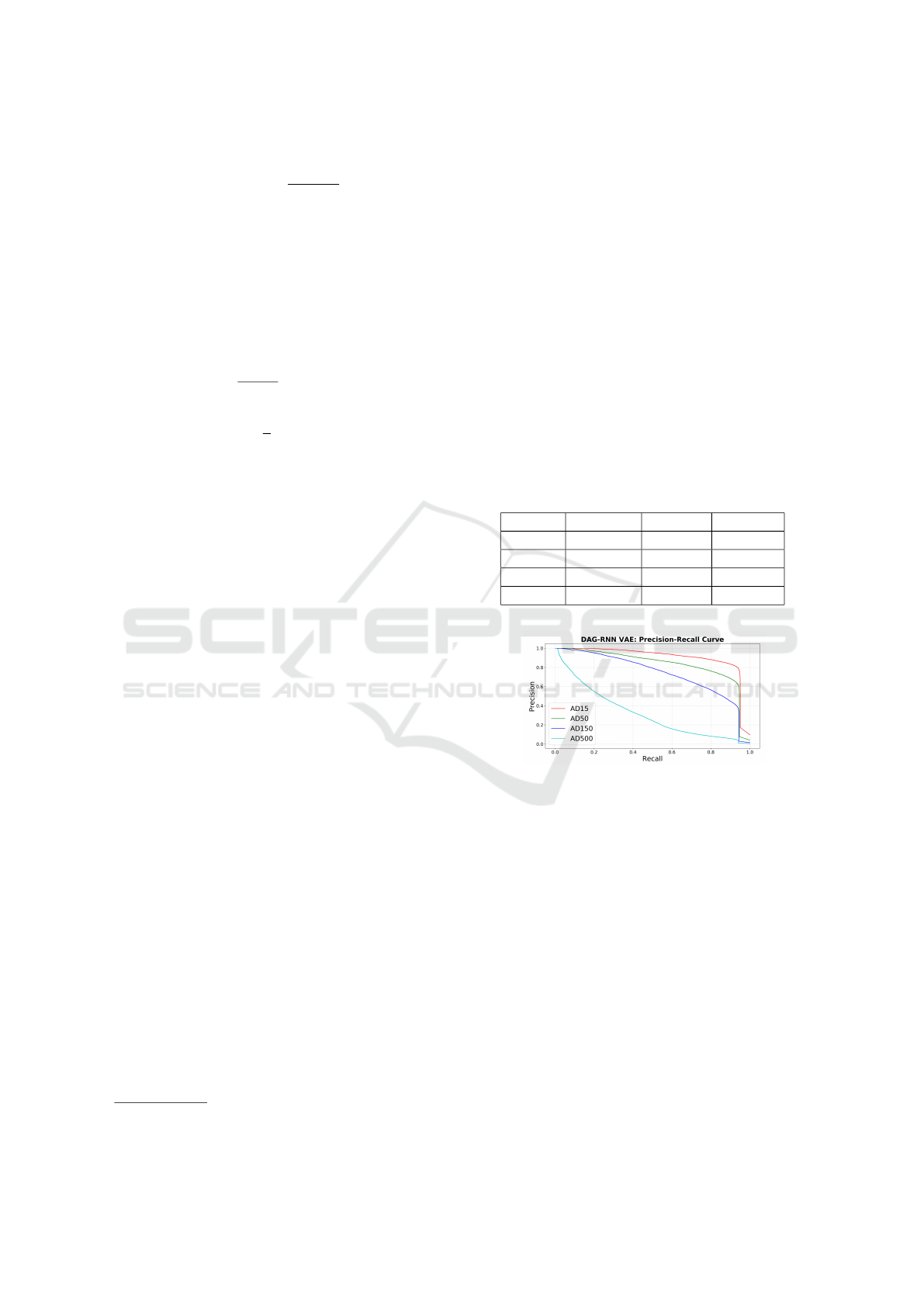
Results of Graph Reconstruction. There are four

sets of results for each of the datasets: AD15, AD50,

AD150 and AD500. Table 2 shows that our model

achieves 80% precision in the testing set of AD15,

AD50, and AD150. However, it only reaches 51%

precision for large datasets of 500 nodes, suggest-

ing that in larger graphs the ability to reconstruct

the graph degrades. The F1-score reaches 84% for

middle-size graphs and is close to 60% for large

graphs. Figure 4 shows a comparison of precision-

recall curves, where it is seen that the largest dataset

AD500 has a drop in performance.

Results suggest that our method can reconstruct

graphs with enough precision up to 150 nodes and are

useful in the generation of new users, but it struggles

with large graphs.

Table 2: Graph reconstruction evaluation metrics.

Dataset Precision Recall F1-score

AD15 80.93% 94.5%6 87.22%

AD50 79.94% 89.48% 84.44%

AD150 80.38% 45.53% 58.13%

AD500 51.85% 72.6% 7 60.52%

Figure 4: Graph reconstruction evaluation comparison with

Precision-recall curves. Only graphs up to 150 nodes have

enough reconstruction precision to be useful.

To compare with GraphRNN we trained with

2,000 nodes and evaluated with 500, extending the

graphs of size 50 with 5 new nodes. Our average

Wasserstein distance is 0.99 (better closer to 0) for

only the extended nodes, which is better than all the

baselines reported in (You et al., 2018). Taking all

the nodes into account (original and new) it is 0.15.

Figure 5 shows an example extended grid.

Results of New Nodes Generation. Table 3 shows

the EVR and MECR metrics for each datasets. EVR

was better for graphs of 50 nodes, with a precision of

80% and an F1-score of 84%. Graphs of 150 and 500

nodes had an F1-score close to 60%, meaning that for

larger graphs we are not generating the same amount

of edges or they are connected differently.

However, with an F1-score 84%, we can expect to

Deep Generative Models to Extend Active Directory Graphs with Honeypot Users

145

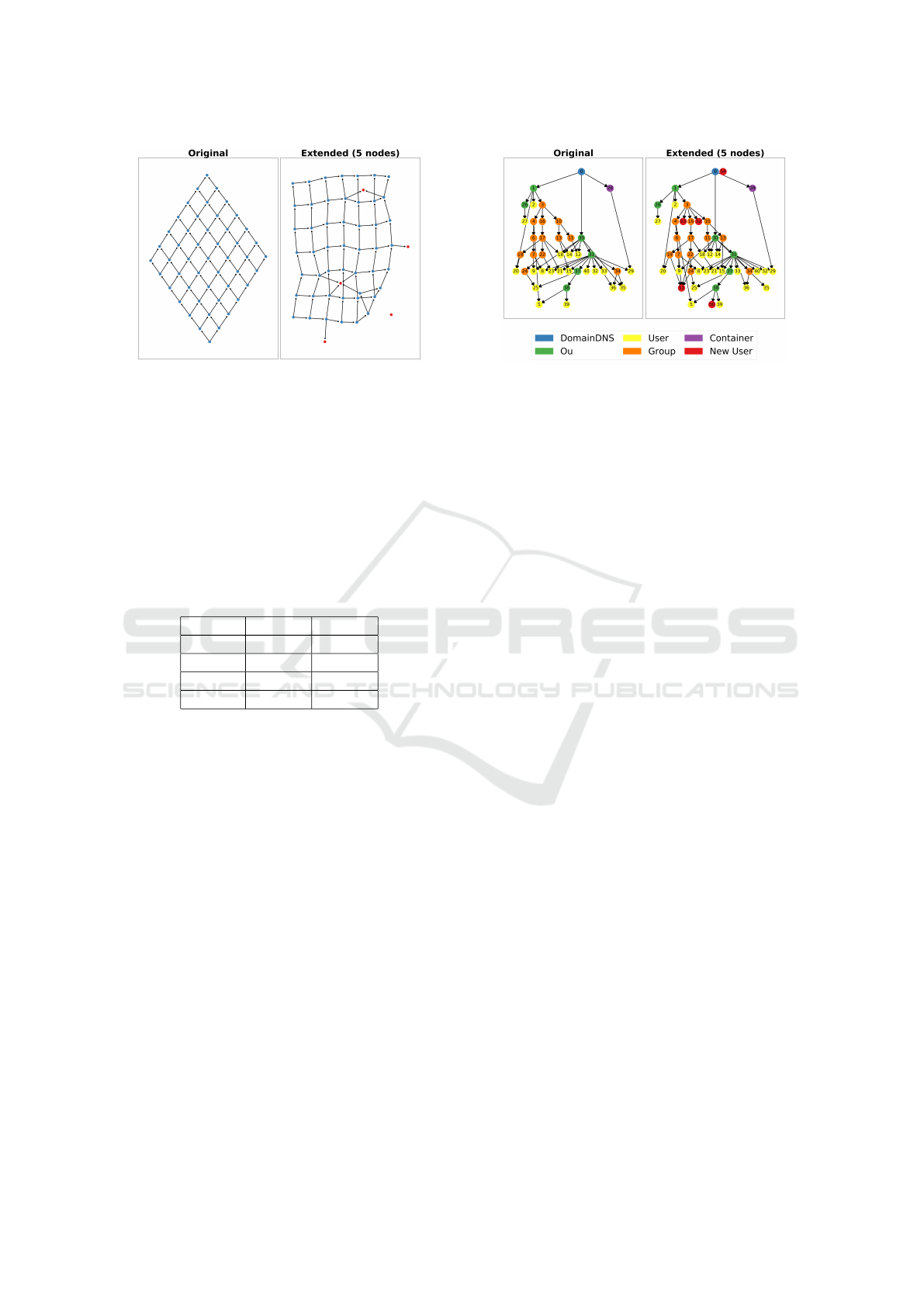
Figure 5: Example of node generation on a 2D grid dataset

from GraphRNN. For the DAG-RNN VAE, we added di-

rectionality and used nodes of the same type. The Wasser-

stein distance of node degree was used in the experiment.

Our method achieved 0.99 which outperforms all baselines

listed in GraphRNN paper. However, the DAG-RNN VAE

does not improve the result of the GraphRNN. The other

two metrics used in that paper are not applicable to our

method.

generate new nodes for graphs of middle size that are

organic enough to be very similar to the other users

of the original graph.

Table 3: Node generation evaluation metrics.

Dataset EVR MECR

AD15 68.38% 77.53%

AD50 72.21% 95.42%

AD150 69.18% 92.42%

AD500 58.86% 95.23%

Our worked on graphs up to 150 nodes with good

results. This was possible because our speciﬁc task of

honeyuser generation needed less precision to work.

Figure 6 is an example of a generated graph of 50

nodes with honeyusers inserted. Newly added users

are depicted in red.

Results of Evaluating Nodes as Honeyusers. This

result has been hard to measure since it is hard to ﬁnd

real attackers to play the game. With ten participants

in the study so far, the results are not statistically sig-

niﬁcant, but they show trends that we expect to con-

tinue for the whole experiment.

For all three questions, both groups (random AD

and generated AD) selected a honeyuser 25% of the

time. At ﬁrst glance, this may seem to suggest that

there is no difference in the generation of edges. How-

ever, for the ﬁrst question participants playing in the

generated AD selected honeyusers 25% of the time,

compared with the participants in the random AD that

selected honeyusers 12.5% of the time. This last re-

sult suggests a possible tendency of attackers towards

Figure 6: Example generated graph (right) from an original

graph (left) from dataset AD50. There are ﬁve user nodes

(ids 50-54 in red) inserted. Node 54 is disconnected from

the graph and is to be discarded.

our generated honeyusers.

Given 100 original and 20 honeyusers, the prior

probability of choosing a honeyuser was 16.6%.

However, for the ﬁrst question, the generated AD

reached 25% of honeyusers hits, suggesting that hon-

eyusers generated by our model may be selected more

than expected. The random AD was below this thresh-

old with 12.5% of honeypot hits.

7 CONCLUSION

We presented a deep learning method that ingests Ac-

tive Directory (AD) structures and generates a similar

structure with inserted honeyusers (fake users). The

method chooses the position of honeyusers in the AD

with a bidirectional topologically sorted DAG-RNN

Autoencoder. The model was evaluated in four ways.

First, by generating similar graphs, showing 80% pre-

cision in graphs up to 150 nodes. Second, by placing

nodes organically, showing a Mean Edge Count Ra-

tio of 92%. Third, by comparing with GraphRNN in

reconstructing grid graphs and being better than base-

lines. Fourth, by generating honeyusers that are at-

tractive to attackers in a public real game, showing

inconclusive results given the small number of partic-

ipants, but with preliminary results that seem to sug-

gest that the nodes placed by our RNN are selected

slightly more.

The contributions of this work are (i) an applica-

tion of DAG-RNN in the cybersecurity domain; (ii)

a free software implementation of DAG-RNN VAE

with GPU acceleration; (iii) a synthetic Active Direc-

tory structure dataset; (iv) a framework for real-life

AD honeyuser evaluation.

Future Work to improve the experiments with

real attackers, to estimate the node type from the

DeLTA 2021 - 2nd International Conference on Deep Learning Theory and Applications

146

embedding, and to include the attractiveness of AD

groups.

ACKNOWLEDGEMENTS

We acknowledge the support of NVIDIA Corporation

with the donation of a Titan V GPU for this research.

We would also like to thank the Stratosphere team for

their support.

REFERENCES

Amizadeh, S., Matusevych, S., and Weimer, M. (2019).

Learning to solve circuit-SAT: An unsupervised dif-

ferentiable approach. In International Conference on

Learning Representations.

Berg, L. (2019). BlueHive.

Bettke, J. and Stewart, J. (2016). DCEPT: An Open-Source

Honeytoken Tripwire.

Case, D. U. (2016). Analysis of the cyber attack on the

ukrainian power grid. Electricity Information Sharing

and Analysis Center (E-ISAC), 388.

Cimpanu, C. (2020a). Fortune 500 company ntt discloses

security breach.

Cimpanu, C. (2020b). Hackers breached a1 telekom, aus-

tria’s largest isp.

Crabtree, J. (2020). Active directory attacks hit the main-

stream. darkreading.com.

de Barros, A. P. (2003). Res: Protocol anomaly detection

ids - honeypots.

Dowling, S., Schukat, M., and Barrett, E. (2018). Using

reinforcement learning to conceal honeypot function-

ality. In ECML/PKDD.

Faraglia, D. (2012). Faker.

Glorot, X. and Bengio, Y. (2010). Understanding the dif-

ﬁculty of training deep feedforward neural networks.

In Proceedings of the International Conference on Ar-

tiﬁcial Intelligence and Statistics (AISTATS’10).

Grimes, R. A. (2006). Honeypots for Windows. Apress.

Guan, S. and Loew, M. (2019). Evaluation of generative

adversarial network performance based on direct anal-

ysis of generated images. In 2019 IEEE Applied Im-

agery Pattern Recognition Workshop (AIPR).

Hagberg, A. A., Schult, D. A., and Swart, P. J. (2008). Ex-

ploring network structure, dynamics, and function us-

ing. In Varoquaux, G., Vaught, T., and Millman, J.,

editors, Proceedings of the 7th Python in Science Con-

ference, pages 11 – 15, Pasadena, CA USA.

Joyce, J. M. (2011). Kullback-Leibler Divergence, pages

720–722. Springer Berlin Heidelberg, Berlin, Heidel-

berg.

Kaluza, M., De Paolis, C., Amizadeh, S., and Yu, R. (2018).

A neural framework for learning dag to dag transla-

tion. In NeurIPS’2018 Workshop.

Karlin, A. R., Bradley, M., Baldwin, M., and Sagir, S.

(2018). What threats does ata look for?

Kingma, D. P. and Ba, J. (2014). Adam: A method for

stochastic optimization.

Kingma, D. P. and Welling, M. (2014). Auto-encoding vari-

ational bayes.

Leita, C., Mermoud, K., and Dacier, M. (2005). Scriptgen:

an automated script generation tool for honeyd. In

21st Annual Computer Security Applications Confer-

ence (ACSAC’05), pages 12 pp.–214.

Liao, R., Li, Y., Song, Y., Wang, S., Nash, C., Hamil-

ton, W. L., Duvenaud, D., Urtasun, R., and Zemel,

R. (2019). Efﬁcient graph generation with graph re-

current attention networks. In NeurIPS.

Lin, T.-Y., Goyal, P., Girshick, R., He, K., and Doll

ar, P.

(2017). Focal loss for dense object detection.

Matsuda, W., Fujimoto, M., and Mitsunaga, T. (2018). De-

tecting apt attacks against active directory using ma-

chine leaning. In 2018 IEEE Conference on Applica-

tion, Information and Network Security (AINS). IEEE.

Metcalf, S. (2015). Red vs. blue: Modern active directory

attacks, detection, & protection.

Microsoft (2015). Advanced Threat Analytics documenta-

tion.

Nurfauzi, R. (2020). Active directory kill chain attack &

defense.

Provos, N. (2003). Honeyd a virtual honeypot daemon.

Simonovsky, M. and Komodakis, N. (2018). Graphvae: To-

wards generation of small graphs using variational au-

toencoders.

Tian, W., Ji, X.-P., Liu, W., Zhai, J., Liu, G., Dai, Y.,

and Huang, S. (2019). Honeypot game-theoretical

model for defending against apt attacks with limited

resources in cyber-physical systems. ETRI Journal,

41(5):585–598.

Valicek, M., Schramm, G., Pirker, M., and Schrittwieser, S.

(2017). Creation and integration of remote high inter-

action honeypots. In 2017 International Conference

on Software Security and Assurance (ICSSA), pages

50–55. IEEE.

Vazarkar, R. (2016). Sharphound.

Whittacker, Z. (2019). Hackers went undetected in citrix’s

internal network for six months.

You, J., Ying, R., Ren, X., Hamilton, W. L., and Leskovec,

J. (2018). Graphrnn: Generating realistic graphs with

deep auto-regressive models.

Zetter, K. (2014). Sony got hacked hard: What we know

and don’t know so far.

Deep Generative Models to Extend Active Directory Graphs with Honeypot Users

147