UAV Inspection of Large Components: Indoor Navigation Relative to

Structures

Martin Sch

orner

, Michelle Bettendorf, Constantin Wanninger

, Alwin Hoffmann

and Wolfgang Reif

Institute of Software and Systems Engineering, Augsburg University, Universit

atsstraße 6a, Augsburg, Germany

Keywords:

Inspeciton of Large Components, UAVs, Adaptive Navigation, Sensor Fusion.

Abstract:

The inspection of large structures is increasingly carried out with the help of Unmanned Aerial Vehicles

(UAVs). When navigating relative to the structure, multiple data sources can be used to determine the position

of the UAV. Examples include track data from an installed camera and sensor data from the orientation sensors

of the UAV. This paper deals with the fusion of this data and its use for navigation alongside the structure. For

the sensor fusion, a concept is developed using a Kalman ﬁlter and evaluated simulatively in a prototype. The

calculated position data are also fed into a vector ﬂight control system, which dynamically calculates and ﬂies

a trajectory along the component using the potential ﬁeld method. This is done taking into account obstacles

detected by the onboard sensors of the UAV. The established concept is then implemented with the Robot

Operating System (ROS) and evaluated simulatively.

1 INTRODUCTION

The inspection of large structures using UAVs is be-

coming increasingly popular. Applications include

the inspection of railway tracks (AG, ), aircraft (Sap-

pington et al., 2019) or the inspection of ship hulls

in dry docks (Englot and S. Hover, 2014). A less

common application is the inspection of large com-

ponents in production. In previous work, we already

covered the derivation of a route through inspection

points based on a list of part positions (Wanninger.

et al., 2020). The next step is ﬂying a trajectory that

visits all points on the route.

A challenge compared to outdoor ﬂights is, that

the usual methods for determining position, such as

GPS, work poorly or not at all in a production hall.

This requires the use of other sensor data to success-

fully determine the UAV’s position. Since external

camera- or radar-based tracking systems are expen-

sive and complex to set up, the work focuses on sen-

sors that can be installed on the UAV. On the one hand,

the inertial measurement unit (IMU) of the UAV itself

allows for computing a position through odometry.

https://orcid.org/0000-0001-6237-222X

https://orcid.org/0000-0001-8982-4740

https://orcid.org/0000-0002-5123-3918

https://orcid.org/0000-0002-4086-0043

On the other hand, its inspection camera can be used

to orient itself relative to the component. The map-

ping between the camera image and the real world is

not presented in this paper. Problematic parameters

such as deviations or latency are simulated. These

sensor data are fused in our approach to obtain a more

accurate and stable position estimate.

We use this position data to ﬂy the UAV au-

tonomously to inspection points calculated in a pre-

vious step. The points are not always approached di-

rectly, but a route is calculated with the help of the

obstacle detection sensors of the UAV, which avoids

unforeseen obstacles along the way. For this purpose,

the potential ﬁeld method (Koren et al., 1991) is used,

in which the UAV is attracted to the nearest target

point (global minimum) and repelled by detected ob-

stacles (maxima).

The contribution of this paper can be summarized as

follows:

• A concept for the fusion of IMU data with camera

tracking data to realize an optimal position esti-

mation relative to a component.

• Adaptive navigation of the inspection UAV rela-

tive to the inspected part with reaction to obstacles

In the following sections, related work on the subject

of inspection by UAVs is presented before the concept

for sensor fusion and dynamic navigation is explained

Schörner, M., Bettendorf, M., Wanninger, C., Hoffmann, A. and Reif, W.

UAV Inspection of Large Components: Indoor Navigation Relative to Structures.

DOI: 10.5220/0010556301790186

In Proceedings of the 18th International Conference on Informatics in Control, Automation and Robotics (ICINCO 2021), pages 179-186

ISBN: 978-989-758-522-7

179

in more detail. Subsequently, the implementation of

the concept is discussed and the results of the evalua-

tion are presented. Finally, a conclusion is drawn and

the further procedure is explained.

2 RELATED WORK

For adaptive navigation, different approaches are con-

sidered below, which support both orientation to ob-

jects and sensor fusions.

In the paper by McAree et al (McAree et al.,

2016), a semi-autonomous UAV is used for structural

inspections. The UAV is equipped with a laser dis-

tance sensor to keep a safe distance from the struc-

ture to assist the pilot. For the assistance feature, the

robotics framework Robot Operating System (ROS)

was used in combination with the simulation environ-

ment Gazebo. For the full automatic inspection pre-

sented in this paper, ROS is also adopted as the basis.

In (Kawabata et al., 2018) and (Mohta et al.,

2018), a depth imaging camera is used instead of a

laser sensor, which also provide 3-dimensional map-

ping of the infrastructure using Simultaneous Local-

ization and Mapping (SLAM). This concept is in-

tended to counteract inaccuracies of the GPS signal

in the proximity of infrastructures. However, navi-

gation is based on a two-dimensional mapping of the

environment. The solution of T. Zhang et al. (Zhang

et al., 2014) also uses SLAM, but in combination with

Monte Carlo simulation. Navigation also takes place

in 2-dimensional space with a laser sensor. The sonar

sensor is only used for the detection of glass.

In the work of L. V. Santana et al. (Santana et al.,

2014), multiple sensors are fused by a simple Kalman

ﬁlter for position tracking. The odometric data of the

UAV and an ultrasonic sensor are used. On the oppo-

site side, the advantages of an extended Kalman ﬁlter

for nonlinear acceleration in the ﬁeld of UAVs is pre-

sented by Belokon et al.(Zolotukhin et al., 2013). In

this project, a trajectory with an average deviation of

0.2m could be ﬂown indoors with only one camera in

combination with UAV odometry. In contrast, a simi-

lar project by Shen et al. (Shen et al., 2013) achieves

an average deviation of 0.5 m with stereoscopic cam-

eras, but at a speed of 4 m/s.

This paper combines the sensor fusion of a simu-

lated tracking camera with the odometry of a copter

and complements it with an adaptive collision detec-

tion and avoidance strategy in an indoor szenario.

3 CONCEPT

In our use case, we assume that a larger structure in a

production hall is to be inspected by a UAV. For this

purpose, the UAV must ﬂy to a sequence of inspection

points from which it can examine relevant parts of the

structure (Wanninger. et al., 2020). In the following,

we ﬁrst give an overview of the overall concept for

ﬂying this sequence of points. Then the individual

components of the architecture are explained in more

detail. These include the determination of the posi-

tion without external sensors and the navigation to the

respective inspection points while avoiding collisions

with obstacles.

3.1 Architecture Overview

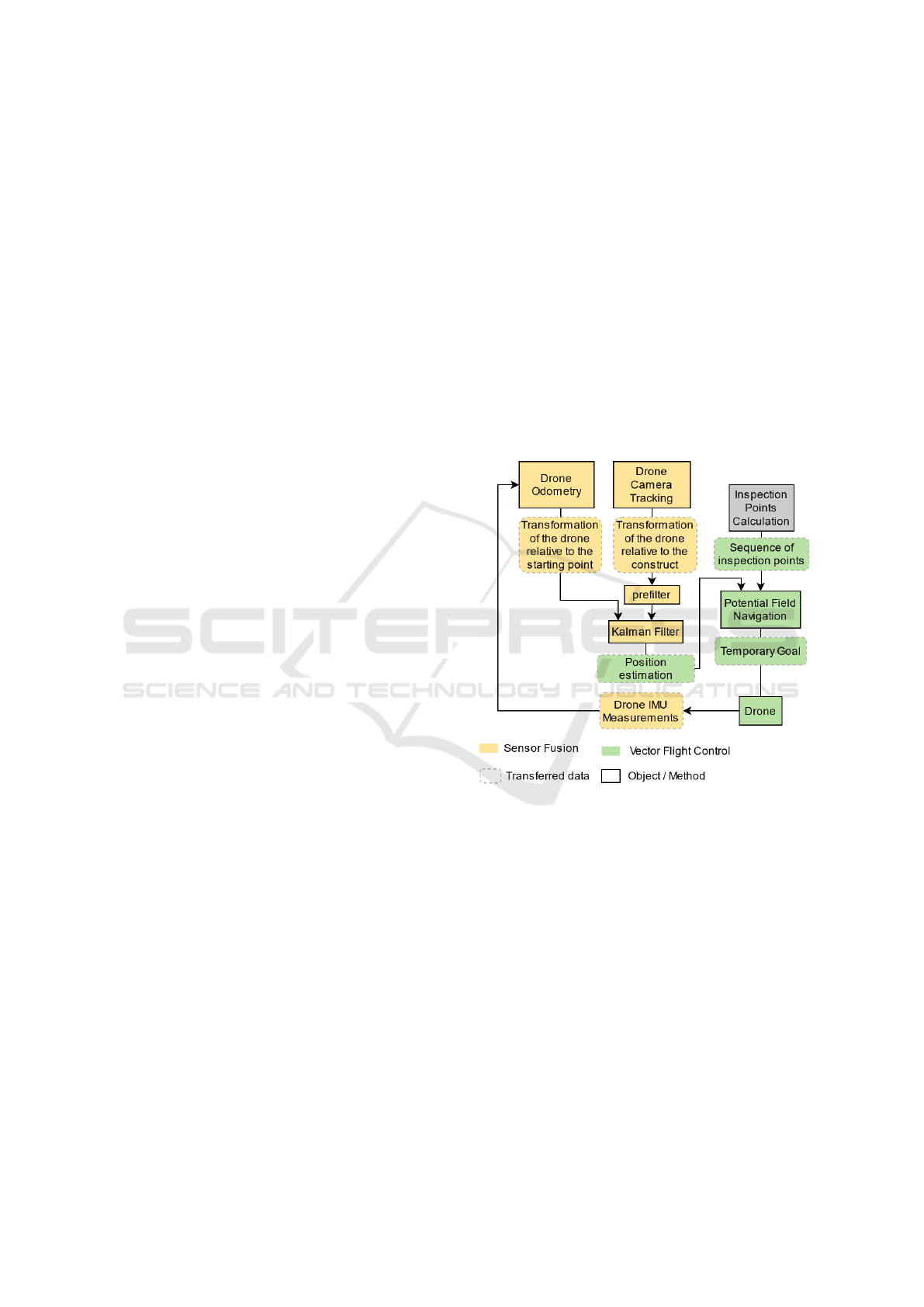
Figure 1: Sensor data of the camera tracking and the drone

odometry are fed to the Kalman ﬁlter which uses these val-

ues to estimates a new position. The estimated position is

used for the potential ﬁled navigation.

The overall architecture of the system can be split

into two interconnected parts (see Fig. 1), the sen-

sor fusion (green) and the navigation system (yel-

low). The IMU provides the estimated position of

the UAV relative to the starting point. Additionaly

the inspection camera can be used to get position in-

formation relative to the inspected structure through

optical tracking algorithms (see (Shen et al., 2013),

(Mohta et al., 2018)). Data from the two input sources

can be used as input for the Kalman ﬁlter (Wan and

Van Der Merwe, 2000), which in turn outputs a more

accurate position estimation. In this paper, a normal

Kalman ﬁlter is used instead of an EKF or UKF (Wan

and Van Der Merwe, 2000) because after lineariza-

ICINCO 2021 - 18th International Conference on Informatics in Control, Automation and Robotics

180

tion, the accuracy of the linearized system is sufﬁcient

for our use case as shown in the evaluation. The po-

sition estimation is used as measured process variable

for the vector ﬂight control. The ﬂight control iterates

over a set of inspection points and generates tempo-

rary setpoints to navigate through the potential ﬁeld

towards the next point. The UAV then feeds back

its IMU data to the Kalman ﬁlter and new camera

tracking data is continuously generated to complete

the control loop.

3.2 Sensor Fusion of UAV Odometry

and Camera Tracking Data

The aim of sensor fusion is to combine different sen-

sor and tracking data to produce a more accurate posi-

tion estimate. The position should not be determined

in a global coordinate system, but in relation to the

component. For this purpose, the IMU data of the

UAV as well as the position determined by camera

tracking are used in our example. The odometry data

provides the transformation from the starting point of

the UAV to its current location and has a relatively

steady course without jumps. However, the deter-

mined position drifts from the actual value over time

due to the dual integration of the IMU’s accelerome-

ter data. Camera tracking of the camera installed on

the UAV determines the position of the UAV relative

to the viewed component. A drift does not occur with

visual tracking. However, under poor visibility con-

ditions, the tracking can brieﬂy output incorrect posi-

tions and thus lead to jumps in the position data. To

combine the advantages of both sensors and to miti-

gate their disadvantages as far as possible, we use a

Kalman ﬁlter to combine the two measured transfor-

mations. Due to the fact that the acceleration of the

UAV is non-linear, the system has to be linearized

in order to be used in conjunction with a standard

Kalman ﬁlter. For the linearization, the mean velocity

for each axis direction (x, y, z) as well as the rota-

tional velocity around the yaw axis will be calculated

in every step. As shown below using the velocity of

the x-axis as an example, the velocities are calculated

by dividing the change in position from time t to (t +

T) by the time difference since the last update (T).

x(t + T ) − x(t)

(1)

The linearization of y, z and yaw is performed analo-

gously. The estimated position from the Kalman ﬁlter

is then used for the trajectory planning.

3.3 Vector Flight Control

In this project, a feasible path which is as short as

possible and collision-free has to be computed out of

a sequence of given view points. The planning will be

done online due to the fact, that in later iterations, the

UAV should be able to avoid dynamic obstacles that

occur at runtime. Because of these constraint a vector

ﬂight control based on a computed artiﬁcial potential

ﬁeld (Chen et al., 2016) was used. The controller gen-

erates a potential ﬁeld based on the current goal and

obstacles in the world. The goal represents a strong,

attracting force, whereas any obstacles have repulsive

potentials around them. The general idea is that at

any given point in the potential ﬁeld the goal position

can be reached by following the potential vector at

the UAV’s current position. Static obstacle positions

are either derived from the CAD-File of the assembly

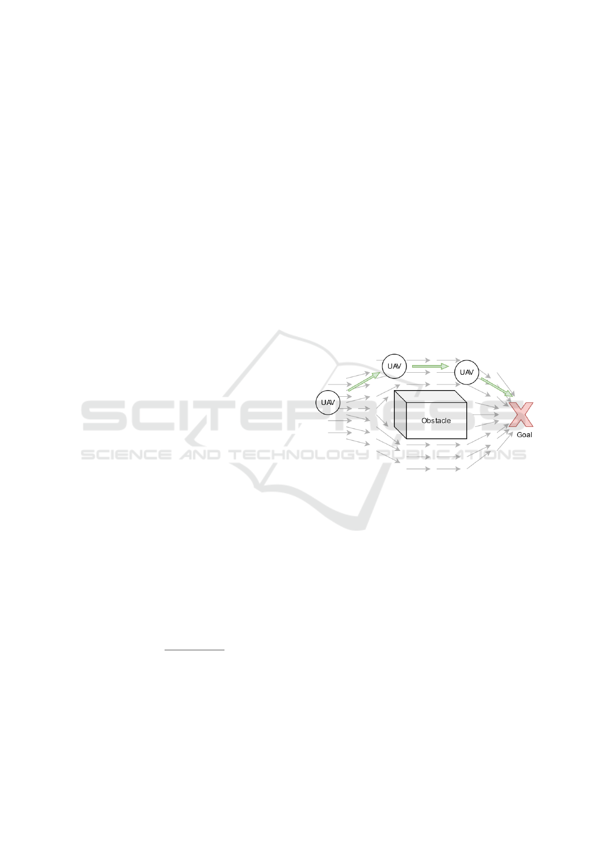
or deﬁned manually. Figure 2 shows an example of

a UAV navigating to a goal point around a static ob-

stacle In this example, the attracting potential of the

Figure 2: UAV navigating around an obstacle in a potential

ﬁeld.

goal pulls the UAV to the left. The obstacle between

the UAV and the goal alter the potential ﬁeld in a way

that causes the UAV to ﬂy around it. This method

works great with obstacles that are known in advance

(e.g. the inspected structure and its ﬁxtures, walls...)

In order to react to dynamic obstacles like people

or tool carts, an extension of this strategy is needed.

Many UAV have onboard collision avoidance sensors

that can detect obstacles in the surroundings of the

UAV. In order ﬂy around these obstacles, the collision

avoidance data can be used to dynamically add obsta-

cles to the potential ﬁeld and recalculate the potentials

based on the new obstacles. By doing this, the UAV

avoids previously known and unforeseen obstacles.

One drawback of the potential ﬁeld method is that

local minimum traps can appear. The goal should al-

ways be the global minimum. However, local min-

ima can occur and if the UAV gets pulled into one

of these minima by the potential, it gets stuck there.

UAV Inspection of Large Components: Indoor Navigation Relative to Structures

181

For solving this issue, we ﬁrst detect, if the UAV is

stuck in a local minimum by checking if its position

stays within a small area for longer periods of time.

We then generate a random point in space as a new,

temporary goal and adjust the potential ﬁeld to acco-

modate the new goal. The random walk method is

illustrated in ﬁgure 3. The robot is moving in a ran-

dom direction, which does not collide with the obsta-

cle. The UAV then approaches the temporary goal for

a certain amount of time to get out of the local min-

imum (see step 2 of Fig. 3). After some time, actual

destination point is set as the goal again and the UAV

either continues towards it or ﬂies back to the local

minimum. If the UAV ﬂies back to the local mini-

mum, the procedure is repeated until the minimum is

escaped.

If the UAV reaches the same minimum for multi-

ple times, there is a possibility that there is no way to

get out of the local minimum. In this case an abort

scenario can be deﬁned where the UAV returns to its

original starting point and lands after a certain number

of unsuccessfull escape attempts.

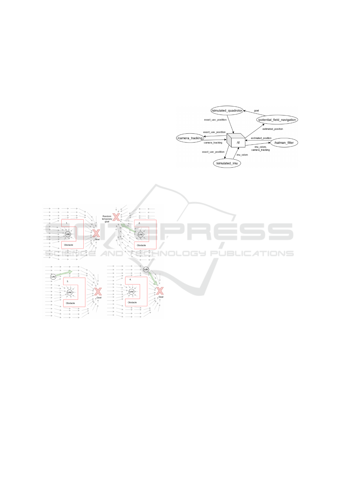
Figure 3: Escaping the local minimum by deﬁning a random

temporary goal.

With these strategies the UAV is able to safely ﬂy

to an inspection point without colliding with its sur-

roundings. Completing a whole inspection is simply

a matter of ﬂying to each of the inspection points of

the given sequence using the method described in this

subsection.

4 IMPLEMENTATION

The following section describes the implementation

of the concept described in 3. It was implemented

using the robotic framework Robot Operating System

(ROS). For the simulation of the UAV we used Ro-

torS (Furrer et al., 2016).

Figure 4: Communication of the implemented ROS nodes.

The camera tracking and imu odometry calculate their sim-

ulated sensor values based of the exact drone position. The

Kalman ﬁlter node uses these positions to create an esti-

mate which is in turn used by the potential ﬁeld navigation

to control the simulated quadrotor.

4.1 Simulated Sensors

In a ﬁrst step, the concept was implemented within a

simulation. Therefore, sensors with similar properties

to their real counterparts were implemented. The sim-

ulated camera tracking data calculates the exact trans-

formation from the UAV to the part to be inspected

and adds “jumps” to the position at randomized times

to simulate tracking erros. This is done by generat-

ing uniformly distributed random distances between

2 and 4 m and adding them to the translation. The

UAV’s odometry is generated by calculating the trans-

formation from the UAV’s starting point to its cur-

rent position. After that an offset that is increasing

by 0.00001 m each step is added to each axis of the

transformation to simulate an error due to drift.

4.2 Kalman Filter

The simulated sensor values are used by the Kalman

ﬁlter to generate a position estimation. Figure 4

shows the Kalman ﬁlter receiving the simulated IMU

and camera tracking sensor data. The camera position

is passed through a pre-ﬁlter that eliminates big jumps

in the camera tracking (see Fig. 1). Since accelera-

tion of the UAV is ﬁnite, it can only move a certain

amount in one control loop. If the change in the po-

sition of the UAV exceeds a predeﬁned threshold, the

measurement is discarded. After this preﬁlter step,

ICINCO 2021 - 18th International Conference on Informatics in Control, Automation and Robotics

182

both sensor inputs are passed to the actual Kalman ﬁl-

ter. The actual Kalman ﬁlter was implemented using

the ﬁlterpy python library (Labbe, 2021).

The state matrix X contains the system states. It

is deﬁned as: [x, vx, y, vx, z, vz, yaw, vyaw]

. The

velocities are calculated by the numerical differenti-

ation of the position. The state transition matrix F is

used to generate the state for the next timestep.

F =







1 dt 0 0 0 0 0 0

0 1 0 0 0 0 0 0

0 0 1 dt 0 0 0 0

0 0 0 1 0 0 0 0

0 0 0 0 1 dt 0 0

0 0 0 0 0 1 0 0

0 0 0 0 0 0 1 dt

0 0 0 0 0 0 0 1







(2)

The measurement martix H is used to connect the

measurements to the states and was deﬁned as a iden-

tity matrix (I). The control transition matrix B is de-

ﬁned as [0,0,0,0]

. For measurement and process

noise R and Q, the value 0.2*I was determined empir-

ically. The system state variable is initialized with the

initial position of the odometry and a velocity of zero.

In each step, a prediction is made using the system

model of the Kalman ﬁlter. Afterwards, new sensor

values of the odometry and the cameratracking are de-

rived from the ROS TF graph. These values are then

used to correct the state estimation of the Kalman ﬁl-

ter. As a last action, the calculated estimated position

of the Filter is published to the TF graph. This posi-

tion is then used by the navigation stack to reach the

predeﬁned inspection points.

4.3 Potential Field Method

Implementation

The inspection points (route) are generated in a previ-

ous step, presented in (Wanninger. et al., 2020) and

loaded by the navigation node which tries to reach

these points sequentially. For reaching each inspec-

tion point the potential ﬁeld method is used, a vec-

tor based navigation with attracting (targets) and re-

pelling (obstacles) potentials. Instead of taking the in-

spection point as the target point, our approach creates

temporary intermediate targets in each iteration that

are approached by the UAV but never reached. This

procedure is necessary because due to proprietary in-

terfaces of the UAV only points and no direction vec-

tors can be submitted. The targets (x) are regularly re-

calculated based on the current potential acting on the

UAV, so that potentially dynamic obstacles can also

be taken into account.

x = x + r ∗ f x (3)

The force in x-direction (fx) is internally deﬁned

cyclically, while the rate (r) is a constant that glob-

ally deﬁnes the distance of the new targets from the

current UAV position and was set to 0.5 in our tests.

The equations for the y and z position are performed

analogously. The resulting temporary target is rede-

ﬁned in ﬁxed time cycles until an inspection point is

reached which can be deﬁned with a deviation, in our

tests this is set to 30cm.

To prevent the UAV from getting stuck in a local

minimum, e.g. a U-shaped obstacle, the random walk

method is utilized. If the UAV has not moved signiﬁ-

cantly within the last time cycle, it is assumed that the

UAV has encountered a local minimum. To get out

of the local minima, new targets are randomly created

each time cycle for the UAV to reach, taking into ac-

count potential repulsive forces. This is repeated until

a target is found that leads out of the minima. Af-

ter leaving the local minima, the distance to the view-

point is recalculated and the last position is updated to

avoid an inﬁnite loop. If no solution to the local min-

ima is found after a deﬁned time, manual interven-

tion is required. When an inspection point is reached,

the process is repeated with the next inspection point

of the route. In a real scenario, the actual inspection

must be performed before proceeding to the next in-

spection point.

5 EVALUATION

The evaluation ist structured in three parts. Initially

the sensor fusion was evaluated by introducing errors

into the camera tracking and imu position. As a sec-

ond step, the vector ﬂight control was tested with us-

ing the exact UAV position. Finally, the position esti-

mated by the Kalman ﬁlter was used to navigate to a

sequence of viewpoints using the vector ﬂight control.

5.1 Sensor Fusion Evaluation

The evaluation of the Kalman ﬁlter is done by man-

ually ﬂying the UAV to predeﬁned points. During

ﬂight, the exact position of the UAV is recorded and

compared to the output of the Kalman ﬁlter. For sim-

plicity we only show one axis of the UAV’s move-

ment. Each graph contains the simulated odometry of

the UAV (blue), the simulated tracking data (green)

and the output of the Kalman ﬁlter (red). The posi-

tions are calculated in relation to the starting position

of the UAV.

Initially a control ﬂight is performed, where both

sensors report the exact UAV position without any er-

rors. Figure 5 shows how the output of the Kalman

UAV Inspection of Large Components: Indoor Navigation Relative to Structures

183

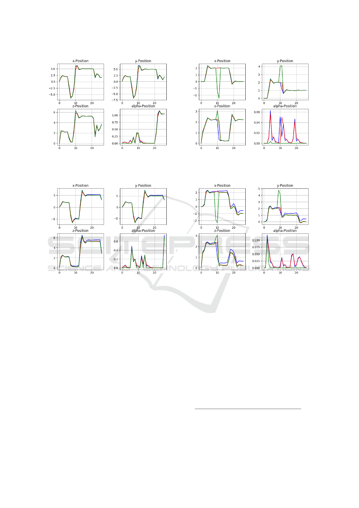
Figure 5: Output of the Kalman ﬁlter (red) with drift-

free imu-position (blue) and jump-free camera tracking data

(green).

Figure 6: Output of the Kalman ﬁlter (red) with drift-

ing imu-position (blue) and jump-free camera tracking data

(green).

ﬁlter follows the sensor data input.

In the next step, we introduced a slowly increas-

ing drift into the IMU position. Figure 6 shows how

the drift only minimally inﬂuences the output of the

Kalman ﬁlter.

We also tested the inﬂuence of jumps in the cam-

era tracking along with clean IMU data (7). Since the

preﬁlter keeps these jumps from getting to the Kalman

ﬁlter, the output remains unaffected of the jump.

Finally, we fed the Kalman ﬁlter the drifting IMU

data and introduced jumps in the camera tracking data

(see Fig. 8). With increasing drift of the IMU posi-

tion, the Kalman ﬁlter trusts the camera tracking data.

When the tracking data cuts out due to the jump, the

estimate deviates towards the drifting IMU position,

but recovers as soon as the tracking data is available

again.

The evaluation of the Kalman ﬁlter shows, that er-

rors like an increasing drift or jumps only inﬂuence

Figure 7: Output of the Kalman ﬁlter (red) with drift-

free imu-position (blue) and jumps in the camera tracking

(green).

Figure 8: Output of the Kalman Filter (red) with drift-

ing imu-position (blue) and jumps in the camera tracking

(green).

the position estimate minimally. Therefore the esti-

mated position can be used for the evaluation of the

vector ﬂight control.

5.2 Vector Flight Control Evaluation

The goal of the vector ﬂight controller is to reach all

inspection points while avoiding static obstacles. For

evaluating the vector ﬂight control, the position esti-

mation from the Kalman ﬁlter is neglected at ﬁrst and

the exact position values are used instead.

In the evaluation scenario the UAV needs to reach

a sequence of three points in 3-dimensional space.

Viewpoint x y z yaw

1 4m 1m 1m 1 degree

2 6m -1m 2m 2 degree

3 2m -2m 3m 1 degree

ICINCO 2021 - 18th International Conference on Informatics in Control, Automation and Robotics

184

The point is considered as reached, if the position

of the UAV deviates less than 0.3

m from the point.

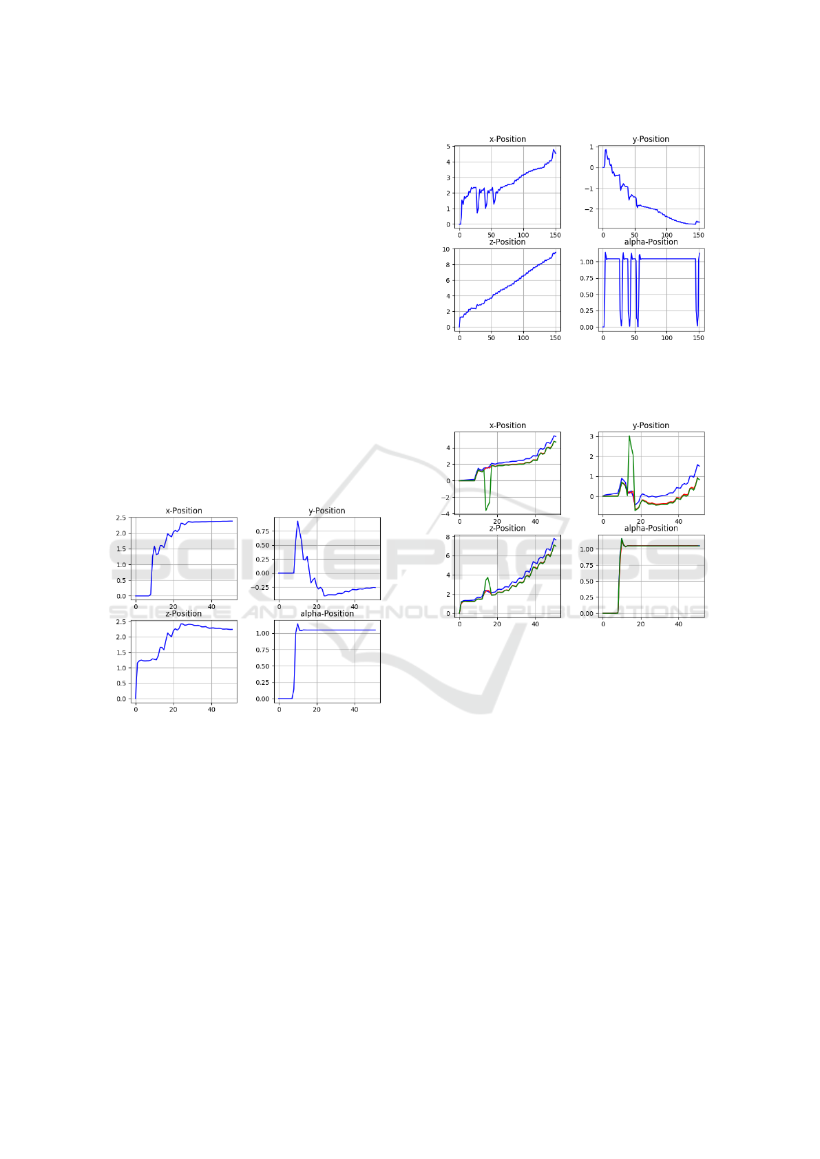
One problem that can occur during navigation is

the UAV getting stuck in a local minimum of the po-

tential ﬁeld The obstacle that causes the minimum in

the potential ﬁeld is shaped like the letter “U” (see

Fig. 3) Figure 9 shows the reaction to a u-shaped lo-

cal minimum trap when only using the potential ﬁeld

method. The UAV is trapped around (2.5, -0.25, 2.5),

because of the u-shaped obstacle. The goal is set to

(5,-3, 10). The UAV can’t escape the trap using the

potential ﬁeld method alone. This is why in the next

pass, the random walk method mentioned in the con-

cept was is performed to escape the minimum. Fig-

ure 10 shows the movement of the UAV with the same

goal as in ﬁgure 9, but with the implemented random

walk method. The random walk method caused the

UAV to ﬂy out of the local minimum, which can be

mainly seen in the x position in ﬁgure 10. It took the

random walk strategy three tries to escape the local

minimum completely. After that, the potential ﬁeld

method was used again to reach the acutal goal with-

out colliding with any obstacles.

Figure 9: UAV stuck in a local minimum at (2.5, -0.25, 2.5).

5.3 Evaluation of the Combined

Architecture

After evaluating the sensor fusion and the navigation

separately, a ﬁnal test was used to evaluate the com-

bination of the two procedures. The UAV was given

multiple goals to ﬂy to sequentially while using the

position estimation generated by the Kalman ﬁlter.

The ﬁlter was fed with a drifting IMU position and

tracking data that had jumps in it. Figure 11 shows

that the ﬁltered position (red) is just slightly affected

by the drift in the odometry data (blue) or the jump

in the camera tracking (green). Despite the two poor

input signals, the UAV manages to reach all targets

within the speciﬁed precision of 0.3

Figure 10: UAV using the random walk method to escape

the local minimum at (2.5, -0.25, 2.5) by ﬂying towards a

random temporary goal before continuing to the actual goal

at (5,-3, 10).

Figure 11: UAV ﬂying to multiple viewpoints while getting

its position from faulty sensor data.

The evaluation has shown that the output of the

Kalman ﬁlter in combination with a preﬁlter for the

cameratracking improves the quality of the position

data compared to the use of a single sensor as a po-

sition source. Our ﬂight control algorithm is capable

of reaching a sequence of waypoints while avoiding

static obstacles, even when using the position estima-

tion provided by the Kalman ﬁlter. It was also demon-

strated, that the algorithm can handle being stuck in a

local minimum of the potential ﬁeld.

6 CONCLUSIONS

This paper covered the inspection of a large structure

like a ship hull. The addressed topics are sensor fu-

sion and vector ﬂight control. To estimate the position

of the UAV the internal IMU and tracking from the in-

spection camera were used. These signals with differ-

UAV Inspection of Large Components: Indoor Navigation Relative to Structures

185

ent fault characteristics were fused by a Kalman ﬁlter.

The camera tracking signal was pre-ﬁltered before it

was sent to the Kalman ﬁlter in order to ﬁlter out harsh

jumps in the tracked position. The estimated position

was fed to a vector ﬂight control based on the poten-

tial ﬁeld method, which allowed the UAV to reach a

sequence of inspection points without colliding with

obstacles in its environment. We also proposed a solu-

tion for the local minimum problem using the random

walk. In our evaluation we demonstrated that fusing

the two sensor values creates an estimate, that is ro-

bust to faulty inputs of one of the sensors. Addition-

ally we demontrated, that our navigation concept al-

lows the UAV to reach a sequence of inspection points

while avoiding surrounding obstacles. Finally it was

shown that the navigation works in conjunction with

the position estimate calculated by the Kalman ﬁlter.

In the future, we are planning on implementing the

proposed algorithms on real hardware. Additionally,

we plan on expanding the navigation to react to dy-

namic obstacles that are not known in advance. This

can be done by dynamically placing obstacles that are

detected by the UAV in the potential ﬁeld and recal-

culating the force vecotor based on the new data. Fi-

nally, using a sensor that tracks the position of the

UAV relative to the part and not relative to a global

coordinate system, could allow the UAV to navigate

relative to the part even when it is in motion. This

would allow inspections of a structure while it is be-

ing craned from one assembly station to another one.

The feasability of this concept will have to be evalu-

ated in future work.

ACKNOWLEDGEMENTS

This work was created in collaboration with Kevin

Dittel, Teoman Ismail, Christian Adorian and

Asa

Odenram from Premium AEROTEC GmbH.

REFERENCES

AG, D. B. Kompetenzcenter multicopter db. last accessed:

08.03.2021.

Chen, Y.-b., Luo, G.-c., Mei, Y.-s., et al. (2016). Uav

path planning using artiﬁcial potential ﬁeld method

updated by optimal control theory. International Jour-

nal of Systems Science, 47(6):1407–1420.

Englot, B. and S. Hover, F. (2014). Sampling-based cov-

erage path planning for inspection of complex struc-

tures. ICAPS 2012 - Proceedings of the 22nd In-

ternational Conference on Automated Planning and

Scheduling.

Furrer, F., Burri, M., Achtelik, M., and Siegwart, R. (2016).

Rotors—a modular gazebo mav simulator framework.

In Robot operating system (ROS), pages 595–625.

Springer.

Kawabata, S., Nohara, K., Lee, J. H., et al. (2018). Au-

tonomous ﬂight drone with depth camera for inspec-

tion task of infra structure. In Proceedings of the Inter-

national MultiConference of Engineers and Computer

Scientists, volume 2.

Koren, Y., Borenstein, J., et al. (1991). Potential ﬁeld meth-

ods and their inherent limitations for mobile robot

navigation. In ICRA, volume 2, pages 1398–1404.

Labbe, R. R. (2021). Filterpy documentation. last accessed:

08.03.2021.

McAree, O., Aitken, J. M., and Veres, S. M. (2016).

A model based design framework for safety veriﬁ-

cation of a semi-autonomous inspection drone. In

2016 UKACC 11th International conference on con-

trol (CONTROL), pages 1–6. IEEE.

Mohta, K., Sun, K., Liu, S., et al. (2018). Experiments

in fast, autonomous, gps-denied quadrotor ﬂight. In

2018 IEEE International Conference on Robotics and

Automation (ICRA), pages 7832–7839. IEEE.

Santana, L. V., Brandao, A. S., Sarcinelli-Filho, M., and

Carelli, R. (2014). A trajectory tracking and 3d po-

sitioning controller for the ar. drone quadrotor. In

2014 international conference on unmanned aircraft

systems (ICUAS), pages 756–767. IEEE.

Sappington, R. N., Acosta, G. A., Hassanalian, M., et al.

(2019). Drone stations in airports for runway and air-

plane inspection using image processing techniques.

In AIAA Aviation 2019 Forum, page 3316.

Shen, S., Mulgaonkar, Y., Michael, N., and Kumar, V.

(2013). Vision-based state estimation and trajectory

control towards high-speed ﬂight with a quadrotor. In

Robotics: Science and Systems, volume 1, page 32.

Citeseer.

Wan, E. A. and Van Der Merwe, R. (2000). The un-

scented kalman ﬁlter for nonlinear estimation. In Pro-

ceedings of the IEEE 2000 Adaptive Systems for Sig-

nal Processing, Communications, and Control Sym-

posium (Cat. No. 00EX373), pages 153–158. Ieee.

Wanninger., C., Katschinsky., R., Hoffmann., A., Sch

orner.,

M., and Reif., W. (2020). Towards fully automated

inspection of large components with uavs: Ofﬂine

path planning. In Proceedings of the 17th Interna-

tional Conference on Informatics in Control, Automa-

tion and Robotics - Volume 1: ICINCO,, pages 71–80.

INSTICC, SciTePress.

Zhang, T., Chong, Z. J., Qin, B., et al. (2014). Sensor fu-

sion for localization, mapping and navigation in an in-

door environment. In 2014 International Conference

on Humanoid, Nanotechnology, Information Technol-

ogy, Communication and Control, Environment and

Management (HNICEM), pages 1–6.

Zolotukhin, Y. N., Kotov, K. Y., Mal’tsev, A., et al. (2013).

Using the kalman ﬁlter in the quadrotor vehicle tra-

jectory tracking system. Optoelectronics, Instrumen-

tation and Data Processing, 49(6):536–545.

ICINCO 2021 - 18th International Conference on Informatics in Control, Automation and Robotics

186