Modeling, Analysis and Control of COVID-19 in Italy: Study of
Scenarios
Paolo Di Giamberardino
a
, Rita Caldarella and Daniela Iacoviello
b
Dept. Computer, Control and Management Engineering Antonio Ruberti, Sapienza University of Rome,
via Ariosto 25, 00185 Rome, Italy
Keywords:
COVID–19, Epidemic Model, Containment Measures Identification, Analysis of Scenarios.
Abstract:
Since the beginning of 2020 in few weeks all the world has been interested by the pandemic due to SARS-
CoV 2, causing more than 3 millions of dead people and more than 146 millions of infected patients. The
virus moves with people and the most effective containment measure appears to be the severe lockdown; on
the other hand, for obvious social and economic reasons, it can not be applied for long periods. Moreover,
the increasing knwoledge on the virus and on its trasmission modes suggested various strategies, such as the
use of masks, social distancing, disinfection and the fast identification of infected patients, up to the recent
vaccination campaign. In this paper, the COVID-19 spread is studied referring to the Italian situation; the
control actions introduced during 2020-2021 are identified in terms of their actual effects, allowing to study
possible intervention scenarios.
1 INTRODUCTION
The COVID-19 emergency has been changing the en-
tire world everyday life, resulting in more than 2.5
millions of dead people and more than 114 millions of
infections, (World Health Organization, 2021). The
most effective containment measures is the social dis-
tancing, applied by means of lockdown, masks wear-
ing, general reduction of mobility and situations of
encounter between people. Nevertheless, the lock-
down, especially in the hard modality, can not be ap-
plied for long periods, both for economic and social
reasons; therefore, a combination of different mea-
sures aiming at reducing the virus transmission is cur-
rently applied by most of the countries. A great effort
has been devoted to understand the virus transmission
modalities as well as to predict the virus diffusion de-
pending on different control actions. Mathematical
modeling of epidemics generally refers to a compart-
mental framework, in which the population is parti-
tioned into classes, depending on their condition with
respect to the infection: the class S of the susceptible
subjects, including the healthy part of the population;
the compartment E of the exposed individuals, i.e. the
subjects in the incubation period; they are infected
but not yet infective; the compartment I of the in-
a
https://orcid.org/0000-0002-9113-8608
b
https://orcid.org/0000-0003-3506-1455
fected patients that can infect the susceptible individ-
uals; the class R of the removed subjects that includes
individuals immunized because healed from the virus
or vaccinated. This kind of basic model is usually re-
ferred as SEIR; for the peculiarities of COVID-19 in
some cases it has been enriched with other classes; for
example, in the SIDART HE model, (Giordano et al.,
2020), the infected patients are discriminated also de-
pending on the severity of their symptoms. In (Tang
et al., 2020), a quite rich model is proposed, including
groups of pre-asymptomatic infectious, hospitalized,
quarantined susceptible, isolated exposed and isolated
infected. Moreover, the pandemic characteristics of
the disease motivate analysis where geographical dis-
placements are considered, as in (Wu et al., 2020).
Other models investigate an important characteris-
tic of COVID-19 related to the greater sensitivity of
the older age groups to the virus, (O’Driscoll et al.,
2020; Di Giamberardino et al., 2020; Colombo et al.,
2020). In (Radulescu et al., 2020) it is assessed the
efficiency and effectiveness of the main control mea-
sures (closures, mobility restrictions, social distanc-
ing), in a sustainability context. This represents one
of the main challenge of all the Governments that
are trying to preserve the population health and the
social/economic aspects of such containment mea-
sures. Since December 2020, vaccination campaign
has started all over the world giving hope of a re-
Di Giamberardino, P., Caldarella, R. and Iacoviello, D.
Modeling, Analysis and Control of COVID-19 in Italy: Study of Scenarios.
DOI: 10.5220/0010555906770684
In Proceedings of the 18th International Conference on Informatics in Control, Automation and Robotics (ICINCO 2021), pages 677-684
ISBN: 978-989-758-522-7
Copyright
c
 2021 by SCITEPRESS – Science and Technology Publications, Lda. All rights reserved
677

turn to normal life. The technical and logistic diffi-
culties of applying massive vaccination campaign to
reach the herd immunity still require a coordination
with the other containment measures. The aim of this
paper is to consider the model of COVID-19 evolu-
tion proposed in ((Di Giamberardino and Iacoviello,
2021)) and (Di Giamberardino et al., 2020), to iden-
tify the main control actions applied during this first
year of pandemic in Italy and to study different sce-
narios. It will be stressed that all the available real
data regarding the number of infected patients are in-
fluenced by the application of the containment mea-
sures; moreover, it is important to identify mathemat-
ically the actions corresponding to the main contain-
ment measures as they are applied by the population.
The paper is organized as follows; in Section 2, the
considered mathematical model is recalled and anal-
ysed preserving the control actions presence and ef-
fects. In Section 3, the peculiarities of the available
data are discussed and the identification procedure is
proposed; numerical results are presented in Section
4, with the analysis of possible scenarios, while con-
clusions are in Section 5.
2 THE MATHEMATICAL MODEL
The mathematical model used in this paper is the one
proposed in (Di Giamberardino and Iacoviello, 2021;
Di Giamberardino et al., 2020), with the introduc-
tion of all the possible (and now) available contain-
ment measures, from the social distancing to the vac-
cination campaign. The classical SEIR model is en-
riched with the class Q of subjects isolated because
waiting the results of the swab test, and to split the
class of infected people into the category of undiag-
nosed patients I
u
(infected and infectious, unaware
of their condition) and the category of infected di-
agnosed ones I
d
(hospitalized or anyway isolated, re-
quiring assistance). The six dimensional system pro-
posed is
˙
S = B − β(1 − u
2
)SI
u
+ bnQ + cnu
5
Q
−au
1
S − d
S
S − vu
6
S (1)
˙
E = β(1 − u
2
)SI
u
− au
1
E − kE −d
E
E (2)
˙
I
u
= kE − au
1
I
u
− h
1
I
u
− h
2
I
u
− d
I
u
I
u
(3)
˙
I
d
= h
1
I
u
+ h
1
(1 − n)Q + c(1 − n)u
5
Q
−(γ + ηu
3
)I
d
− d
I
d
(1 − u
4
)I
d
(4)
˙
Q = au
1
(S + E +I
u
) − bnQ − h
1
(1 − n)Q
−cu
5
Q − d
Q
Q (5)
˙
R = h
2
I
u
+ (γ + ηu
3
)I
d
− d
R
R + vu
6
S (6)
The parameters introduced in (1)–(6) have the follow-
ing meanings, (see also (Di Giamberardino and Ia-
coviello, 2021) for more details). The death rates in
each class, possibly different each other, are denoted
by the d
∗
terms. B represents the constant rate of new
incoming individuals; parameter β is the contact rate,
including information of various factors, the aggres-
siveness of the virus, the frequency of the contacts be-
tween individuals and their duration. The natural tran-
sition between classes are weighted by the quantities
k, h
1
, h
2
and γ.Parameter n is related to the fraction
of subjects that have a negative response from the test
campaign; it can be estimated as
S(t)
S(t)+E(t)+I
u
(t)
and it
is connected with b. The parameter b is the rate of
return from the quarantine to the health susceptible
people; from the Q class, after the results of the test,
negative with probability n or positive for the remain-
ing 1−n, the transition to the corresponding class oc-
curs at rate c. Also the control actions are considered.
u
1
aims to stimulate, or force, a test campaign on the
population, with an efficacy coefficient a. u
2
models
the isolation indications to reduce possible contagious
sources; this isolation, that does not involve medical
structures, acts on the factor β for the part responsi-
ble of the frequency of individual contacts. The con-
trol u
3
represents the therapy action devoted directly
to counteract the virus by means of antiviral drugs
with coefficient of effectiveness η. u
4
is the therapy
actions aiming at reducing the side–effects of the in-
duced cardio–respiratory diseases; it is introduced as
a direct contribution to reduce the mortality rate and
it is bounded between zero (no therapy) and 1 (all in-
dividuals kept alive during the infection course). u
5
takes into account various kind of constraints influ-
encing the tests policy. u
6
regards the vaccination
strategy, with coefficient v denoting its efficiency.
2.1 Model Analysis
Since the very beginning of the epidemic alarm, in-
creasing containments measures have been applied
by all the governments; therefore, the available real
data concerning the epidemic spread are affected by
time–varying control actions aiming at reducing its
effects. This consideration suggested to include all
the controls u
i
, i = 1, ..., 6, in the model analysis,
thus determining how the equilibrium points are influ-
enced by the interventions, both in their number and
in their stability properties. The following notations
are adopted, for sake of simplicity in the formulation,
with obvious meaning of the symbols
•
¯
β(t)=β(1 − u
2
(t))
•
¯
γ(t)=γ + ηu
3
(t)
•
¯
d
I
d
(t)=d
I
d
(1 − u
4
(t))
• m
1
(t) = au
1
(t) + d
S
+ vu
6
(t) = ¯a(t)+d
S
+ ¯v(t) >0
ICINCO 2021 - 18th International Conference on Informatics in Control, Automation and Robotics
678

• m
2
(t)=au
1
(t) + k + d
E
= ¯a(t)+k + d
E
>0
• m
3
(t)=au
1
(t) + h
1
+ h
2
+d
I
u
= ¯a(t)+h
1
+ h
2
+ d
I
u
>0
• m
4
(t)=bn + cu
5
(t)n= bn + ¯c(t)n > 0
• m
5
(t)=bn + h
1
(1 − n)+cu
5
(t)+d
Q
= bn + h
1
(1 − n)+ ¯c(t)+d
Q
>0
• m
6
(t)=d
S
+vu
6
(t)= d
S
+ ¯v(t)> 0
To determine the equilibrium points, assuming con-
stant control actions, the second members of the equa-
tions (1)-(6) are put equal to zero, thus determining
the disease-free one (DFE), always present, given
by:
P
e
1
=

S
e
1
E
e
1
I
e
u1
I
e
d1
Q
e
1
R
e
1

T
with E
e
1
= I
u1
= I
d1
= 0 and
S
e
1
=
Bm
5
d
Q
m
1
+ m
4
m
6
(7)
Q
e
1
=
B ¯a
d
Q
m
1
+ m
4
m
6
(8)
R
e
1
=
B ¯vm
5
d
R
(d
Q
m
1
+ m
4
m
6
)
(9)
Note that in the disease free case the probability n of
having negative COVID-19 test (and so to be healthy)
is equal to 1. A second equilibrium point, the endemic
one, may exist, depending on model parameters and
control actions:
P
e
2
=

S
e
2
E
e
2
I
e
u2
I
e
d2
Q
e
2
R
e
2

T
(10)
with
S
e
2
=
m
2
m
3
k
¯
β
E
e
2
=
m
3
k
I
e
u2
Q
e
2
=
¯am
2
m
3
kβm
5
+
¯a
m
5
(
m
3
k
+ 1)I
e
u2
I
e
d2
=
1
¯
γ +
¯
d
I
d
(h
1
I
e
u2
+ (1 − n)(h
1
+ ¯c)Q
e
2
)
All these quantities, with the exception of S
e
2
, depend
on I
e
u2
, and are well defined once I
e
u2
is. Its expression
is given by:
I
e
u2
=
¯am
2
m
3
m
4
+ k
¯
βm
5
B − m
1
m
2
m
3
m
5
¯
β(
¯
βm
2
m
3
m
5
k − ¯am
3
m
4
− ¯akm
4
)
(11)
This solution can be accepted only if positive; by sub-
stituting the definitions of m
i
, i = 1, ..., 5 it can be
easily shown that the denominator is always positive,
whereas the sign of the numerator depends on the con-
dition:
¯
βkBm
5
m
2
m
3
(m
4
m
6
+ d
Q
m
1
)
− 1 > 0 (12)
The existence condition of the endemic equilibrium
point P
e
2
is related to the concept of the reproduction
number, that is the number of secondary cases pro-
duced by one infected subject in a completely sus-
ceptible population during its infectious period. This
indicator, important to have information on the epi-
demic evolution, can be estimated starting from the
real data; a different model based approach implies
the evaluation of the next generation matrix in the
disease free equilibrium, (7), that includes the func-
tions related to vaccination, when possible, and the
test campaign. The computation starts considering in
the dynamics (1)–(6) the classes directly involved in
the spread of the infection, i.e. E, I
u
, I
d
and Q, and
therefore only the equations (2)–(5). By using the
notations with the m
i
, i = 1, . . . , 6, quantities, the re-
duced system (2)–(5) may be written enhancing the
contributions due the infection, F , and the ones due
to changing the health condition, V :

˙
E
˙
I
u
˙
I
d
˙
Q

T
= F − V (13)
where
F =



βSI
u
0
0
0



(14)
V =



m
2
E
−kE +m
3
I
u
−h
1
I
u
− [(h
1
+ ¯c)(1 − n)Q − (
¯
γ + d
I
d
)I
d
]
− ¯a(S + E + I
u
) + m
5
Q



(15)
The variations of F and V with respect to the vari-
ables E, I
u
, I
d
and Q yield the matrices F and V re-
spectively:
F =
∂F
∂(E, I
u
, I
d
, Q)




P
1
e
V =
∂V
∂(E, I
u
, I
d
, Q)




P
1
e
(16)
Under these positions, the reproduction number R is
given by the dominant eigenvalue of the matrix FV
−1
,
in the present case its {1, 1} element; the computation
easily yields:
R =
¯
βkS
e
1
m
2
m
3
(17)
Note that R is the same quantity as in (12), related to
the existence of the endemic equilibrium P
e
2
depend-
ing on its value with respect to the threshold 1. From
(17) it is evident that the introduction of the vacci-
nation, present in the terms m
1
(t) and m
6
(t), reduces
Modeling, Analysis and Control of COVID-19 in Italy: Study of Scenarios
679

the reproduction number; this is in agreement with the
first data of the vaccination campaign in the United
Kingdom. By studying the Jacobian matrix of the sys-
tem (1)–(6), it is possible to establish a stability con-
dition and to link it with the reproduction number R .
In particular, for the disease free equilibrium P
e
1
two
negative eigenvalues,−d
R
and −(
¯
γ +
¯
d
I
d
), are easily
identifiable; for the reduced Jacobian matrix:
˜
J =




−m
1
0 −
¯
βS
e
1
m
4
0 −m
2
¯
βS
e
1
0
0 k −m
3
0
¯v 0 h
1
0




(18)
the characteristic equation evaluated in P
e
1
yields four
roots obtained from the following polynomial:
P(λ) = λ
4
+ N
3
λ
3
+ N
2
λ
2
+ N
1
λ + N
0
(19)
where N
3
= m
1
+ m
2
+ m
3
+ m
5
and the other coeffi-
cients depend on R :
N
2
= m
2
m
3
(1 − R )+ (m
2
+ m
3
)(m
1
+ m
5
)
+ m
1
m
5
− ¯am
4
(20)
N
1
= m
2
m
3
(1 − R )(m
1
+ m
5
)
+ (m
2
+ m
3
)(m
1
m
5
− ¯am
4
) (21)
N
0
= m
2
m
3
(1 − R )(m
1
m
5
− ¯am
4
) (22)
By substituting the expressions of the quantities m
i
,
i = 1, ..., 5, it results the positiveness of m
2
· m
3
and
of m
1
· m
5
− ¯am
4
. Therefore, by using Routh’s argu-
ments, the negativeness of the real parts of the roots
of P(λ) depends on the positiveness of the quantity
1 − R . It is possible to conclude that in this case
only the disease free equilibrium P
e
1
exists and it is
stable. Also in the proposed approach, that includes
the control actions as structural part of the model-
ing, it can be deduced that if the reproduction num-
ber is smaller than 1 there exists a unique equilibrium
point, the disease free equilibrium one, and it is sta-
ble; otherwise, for R > 1, the equilibrium points are
two and the disease free one is not stable any more.
It is useful to stress that, for the assumed choice of
including the control actions in the analysis, both P
e
1
and P
e
2
are influenced by the containment measures.
The disease free equilibrium one, P
e
1
, could be inter-
preted as follows; when a population is in that con-
dition by means of the control actions introduced and
for the model parameters, if the quantity R is smaller
than one then the population will remain near the P
e
1
equilibrium point, without allowing the spread of the
epidemic. Referring to COVID-19 (and therefore as-
suming fixed model parameters) and to the expression
(17) of R , a suitable application of social distancing
(thus acting on
¯
β), of swab tests and quarantine (thus
acting on ¯a and ¯c), medication (acting on
¯
γ) and vac-
cination (control ¯v) would lead the population to the
disease free equilibrium point.
3 CONTROL ACTIONS
IDENTIFICATION
Since the very beginning of the pandemic, it appeared
fundamental the collection of real consistent data, to
be able to understand what was happening in a situa-
tion for which the entire world was unprepared. In
this paper the real data regarding the Italian situa-
tion are considered; they have been downloaded from
the Civil Protection website (Protezione Civile, ): in
particular, it is considered the number of positive pa-
tients I
real
, corresponding to the I
d
ones of this model,
the number of subjects officially recovered R
real
and
the ones dead for the virus direct and indirect effects
D
real
. Due to the presence of asymptomatic subjects,
the last two groups of data correspond to the output
of the I
d
compartments weighted by the recovery (
¯
γ)
and death (
¯
d
I
d
) coefficients respectively. One of the
difficulties in using COVID-19 real data regards the
consistency in their collections, especially in the first
period of the epidemic spread; moreover, due to the
increased awareness of the importance of some infor-
mation (for example, the number of swab tests, or of
hospitalized patients) it has been decided, only with
some delay, to collect new kind of data, that, there-
fore, are not available since the very beginning of the
epidemic emergency. Among the European Nations
the modalities of how deaths are counted are different
(depending on the dominant cause of death) or data
are grouped in different ways. Moreover, some fluc-
tuations in the number of swab tests processed during
the week–ends alter the trend of the number of sub-
jects positive to COVID-19, thus suggesting to use,
as a possible indicator of the course of the pandemic,
the normalized number with respect to the total num-
ber of tests. Some of the parameters introduced in
the proposed model (1)–(6) can be assumed known
from the medical literature, as the incubation time or
the recovery rate; they will be discussed in the next
section. As far as the identification of the control ac-
tions included in the model, note that the contribu-
tion of control u
6
exists only starting from January
2021. The actions, u
i
i = 1, ..., 6, are included in the
variables defined in Subsection 2.1, ¯a(t),
¯
β(t),
¯
γ(t),
¯
d
I
d
(t), ¯c(t), ¯v(t), respectively. Moreover, in order to
improve the quality of the identification and simplify
the numerical implementation, it can be stressed the
relation among the two control actions u
3
and u
4
, and
therefore among the variables
¯
γ(t) and
¯
d
I
d
(t). In the
equation (4) the two contributions related to healing
and to death are assumed separated since they corre-
spond to different therapy actions. Nevertheless, their
effects are strictly related, since a patients can leave
the I
d
compartment only healing or dying; moreover,
ICINCO 2021 - 18th International Conference on Informatics in Control, Automation and Robotics
680

the two controls u
3
and u
4
generally refer to the medi-
cation aspect ascribable to the same kind of resources.
Therefore a unique control parameter can be identi-
fied yielding both the actions; more precisely, it is as-
sumed a relation between u
3
and u
4
:
¯
γ(t) = γ+ ηu
3
(t) = h
3
u
4
(t) (23)
where parameter h
3
is related to the rate of healing
for infected patients. The following cost index is pro-
posed, aiming at fitting the available real data:
J( ¯a,
¯
β,
¯
γ, ¯c, ¯v) =
Z
t
f
t
0
[w
1
(I
N
real
(t) − I
N
model
(t))
2
+w
2
(I
real
(t) − I
d
(t))
2
+ w
3
(R
real
(t) − R
I
d
(t))
2
+w
4
(D
real
(t) − D(t))
2
+ w
5
(V
real
(t) −V(t))
2
]dt (24)
where I
N
model
(t) is the number of new diagnosed infec-
tions obtained by adding the variation of the number
of infected patients, of the recovered and the dead in-
dividuals between two consecutive days; I
N
real
(t) is the
same quantity calculated on real data; R
I
d
(t) are the
subjects recovered from the I
d
compartment R
I
d
(t) =
(γ + ηu
3
(t))I
d
(t) and R
real
(t) the official real value of
healed subjects; D(t) is the number of dead patients
obtained from the model D(t) = d
I
d
(1 − u
4
(t))I
d
(t)
and D
real
(t) the official corresponding quantity; V
real
is the number of subjects vaccinated with the two
doses corresponding to the quantity ¯vS of the model.
The parameters w
i
, i = 1, .., 5 are the weights indi-
cating the relevance of each term in the optimization
procedure. The period considered covers all the pan-
demic year, from the March 2020 to the end of Febru-
ary 2021, in which different and complementary con-
tainment measures have been adopted by the Italian
Government. The main adopted containment mea-
sures may be summarized as follows:
• from February 23 to March 8, 2020: introduc-
tion in the north of Italy of increasing containment
measures;
• from March 9 to May 3, 2020: severe lockdown in
the entire nation, with the suspension of all non–
essential activities; this period is called ”Phase 1”;
• from May 3 to June 10, 2020: almost all the ac-
tivities started again; this period is the ”Phase 2”;
• from June 11 to October 12, 2020: it is the period
with less restrictions; it is the ”Phase 3”;
• from October 13 to November 2, 2020: intro-
duction of increasing containment measures with
mandatory use of mask;
• from November 3 to December 21, 2020: it was
introduced the curfew from 10 pm to 5 am; more-
over it was adopted a classification mechanism of
each region in three classes indicated by colours,
yellow, orange, red, with increasing level of re-
strictions depending on the diffusion of the virus
and of the sanitary situation at territorial level.
This phase could be recalled as the ”Phase of
colours”;
• from December 22, 2020 to January 6, 2021: the
strategy based on the colours was reinforced; all
Italy was in the orange level but it became red in
the holidays;
• from January 7 to February 28, 2021: the strategy
with colours of the period November 3 - Decem-
ber 21 2020 was adopted with reinforced contain-
ment rules.
4 NUMERICAL RESULTS
The data considered in this paper regards the period
February 2020 (the very beginning of data collection)
up to April 2021; the real data used are taken from
the Civil Protection website ((Protezione Civile, )).
First, the model is identified by minimizing the cost
function (24) and determining the functions ¯a,
¯
β,
¯
γ
and ¯c related to the controls, u
1
, u
2
, u
3
, u
5
and u
6
,
considering the simplification in (23). Therefore, it
is possible to establish a correlation between the of-
ficial containment measures applied, and the identi-
fied functions. In fact, generally it is not easy to
”convert” the complexity of any Government actions,
thought as the combination of different containment
measures, into a function, also considering the differ-
ent reactions of the population. Finally, some inter-
esting scenarios are studied. In (1)–(6), some of the
parameters can be considered known, since related
to the population characteristics, and obtained from
the ISTAT website (Istituto Nazionale di Statistica, ):
B = 1.69 · 10
3
; d
S
= d
R
= 2.81 · 10
−5
. Other parame-
ters are assumed known only as mean values, consid-
ering their medical meaning and the estimation given
by the physicians, (Di Giamberardino and Iacoviello,
2021): k =
1
4
; d
E
= d
Q
= d
I
u
= d
S
; d
I
d
=
1
12
; b =
1
14
;
h
1
=
1
5
; h
2
=
1
21
; h
3
=
1
40
. As far as the choice of the
weights in the cost index, with a trial and error pro-
cedure the following values are taken up to Decem-
ber 2020 (when the vaccination was not available):
w
1
= 0.4, w
2
= w
3
= w
4
= 0.2, w
5
= 0; while, after
January 2021 the choices w
1
= 0.4, w
2
= 0.2, w
3
=
w
4
= 0.15, w
5
= 0.1 are adopted. The minimization
of the cost index (24), min
( ¯a,
¯
β,
¯
γ, ¯c)
J( ¯a,
¯
β,
¯
γ, ¯c), with re-
spect to the functions ( ¯a,
¯
β,
¯
γ, ¯c), is implemented by
using the Matlab
R

function fmincon, thus obtaining
the fitting of the real data considered, see Figs.1–3.
In all the figures, the dotted lines indicate the starting
Modeling, Analysis and Control of COVID-19 in Italy: Study of Scenarios
681

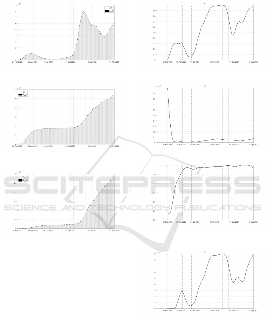
Figure 1: Infected patients I
d
(t) estimated from the model
versus the corresponding real data.
Figure 2: Dead patients D(t) estimated from the model ver-
sus the corresponding real data.
Figure 3: Recovered subjects R
I
d
(t) estimated from the
model versus the corresponding real data.
days of the main containment measures listed in the
previous Section.
It can be noted the general good fitting to the cor-
responding real data of the variables I
d
(t), D(t) and
R
I
d
(t), also in the sudden variations of the total num-
ber of infected patients, in the periods April-May and
November-December 2020. The minimization of the
cost index (24) yields the evolution of the functions ¯a,
¯
β,
¯
γ and ¯c, filtered on a window of 14 days, Figs. 4 -
7.
Besides some fluctuations, due to variability of
real data, it can be noted the general increasing trend
of the strongly related functions ¯a and ¯c, correspond-
ing to the test campaign and the efficiency of the test
policy, in particular from July 2020 to January 2021,
Figs. 4 and 7. The therapy capability, both at reducing
the side-effects of COVID-19, as well as to counteract
Figure 4: Reconstructed evolution of ¯a related to the control
action u
1
(t).
Figure 5: Reconstructed evolution of
¯
β(t) = β(1 − u
2
(t)).
Figure 6: Reconstructed evolution of
¯
γ(t) corresponding the
control action u
3
(t) and u
4
(t) according to the simplifica-
tion in (23).
Figure 7: Reconstructed evolution of ¯c corresponding to the
control action u
5
(t).
the virus, is shown in Fig.6 by means of the function
¯
γ; note, as reasonable and desirable, the increased ca-
pability in contrasting the infection.
The identification of
¯
β(t) is particularly interest-
ing, Fig. 5; the decrement of the identified function
ICINCO 2021 - 18th International Conference on Informatics in Control, Automation and Robotics
682

Figure 8: Reconstructed evolution of ¯v corresponding to the
control action u
6
(t).
¯
β(t) corresponds to an increment of the control u
2
(t).
It models the limitations of the possible contacts be-
tween susceptible subjects and infected patients. Note
that, while up to June (i.e. during the severe lock-
down and the start of Phase 3) the function
¯
β(t) had
low values (and so the control was very effective), in
the summertime the restrictions became less severe,
with an increase of
¯
β(t) that reached its maximum
in October 2020. The negative effects of the corre-
sponding low values of control u
2
(t) were observed
at the end of November with the peak of the sec-
ond epidemic wave, see Fig. 1. Also the first three
months of the vaccination campaign are considered,
Fig. 8; it can be noted, after the middle of Febru-
ary 2021, the monotonic increase in the vaccination
action. It is worth to be stressed that the identified
controls correspond to the actions as they were really
applied by the population. One of the difficulty in
facing this pandemic is to balance the need of stop-
ping the infection and the social/economic problems
involved in the reduction of activities. Therefore, the
choice of ad hoc containment measures, effective but
not too restrictive, represents one of the challenge of
any Government. Another difficulty relies in the fact,
stressed in this paper, that the available data are influ-
enced, since the very beginning of the pandemic, by
the containment measures applied.The availability of
a model that fits the controlled data and identify the
main containment measures, as they were applied by
the population, allows to partially overcome this prob-
lem and study some scenarios. In particular, assuming
the same functions ¯a, ¯c and
¯
γ as at the end of Febru-
ary 2021, the following cases are studied: Scenario
1: introduction, at the beginning of March 2021, of a
severe lockdown, as in the period March 2020- April
2020; Scenario 2: introduction, at the beginning of
March 2021, of mild measures, as in the period July
2020- October 2020; Scenario 3: study the effects of
the application of severe lockdown starting in Octo-
ber 2020. The results obtained in the three cases are
all intuitive from a qualitative point of view; here also
a quantification is possible, providing a support in the
containments measures decision process. In the first
two scenarios, regarding the spring 2021, also a first
small percentage of vaccination effect is included. In
both cases, it is assumed an immunization after an av-
erage period of 60 days (it depends on the kind of
vaccine) and a percentage of population immunized
by vaccination of about 0.05% (it depends on the rate
of administration of the vaccine, on the availability of
doses and on the logistic capability for a mass vacci-
nation campaign). By considering Fig. 9, in which
two opposite strategies are adopted starting in March
2021, it can be seen that with a severe lockdown the
total number of infected patients rapidly decreases in
less than one month, reaching almost the same value
of October 2020. By applying mild containment mea-
sures as in summer 2020, a rapid increase is shown;
the bar plot shows the real trend of infected patients
depending, of course on the containment measures
adopted, as a balance between the two extreme pos-
sible choices. These results confirm the importance
of applying containment measures, despite the vacci-
nation campaign, until the herd immunity is achieved.
In Fig. 10 it is proposed an ex-post analysis of what
could have happened if in November 2020 a severe
lockdown was applied. The attention is focused to
that period since, as seen in Fig.1, it represents the
onset of the second wave, consequence of different
issues: the summertime mild restrictions with trav-
els, the weather conditions, the re-opening of many
activities that implied a reduction of the social dis-
tancing. In Fig. 10 it can be seen that the peak of
infections could have been significantly lower with a
value of infected patients at the end of January re-
duced of about 60%. Obviously, the lockdown low-
ers the curve; nevertheless the modeling approach al-
lows to establish for how long it is advisable to extend
specific control actions. In this paper, the contain-
ment measures are identified as applied by the pop-
ulation; nevertheless, among the possible future de-
velopments, optimal scheduling could be proposed,
as well as resources allocation, taking into account
the limitations under material and logistic points of
view. Moreover, the effects of the vaccination cam-
paign will be included, as well as its relations with the
other containment measures; other scenarios regard-
ing past and future possible choices for the control
actions will be investigated: in the globalized world
pandemic is not an exception and the severe lockdown
could not be the unique solution but should be inte-
grated with strategies able to consider contemporary
different requirements, in a complex framework.
Modeling, Analysis and Control of COVID-19 in Italy: Study of Scenarios
683

Figure 9: Scenario 1 and 2: Comparison of the possible
evolution of the number of diagnosed infected patients I
d
(t)
with respect to different strategies and real data.
Figure 10: Scenario 3: Comparison of the real evolution of
the number of diagnosed infected patients I
d
(t) with the one
obtained in the hypothetical scenario 3.
5 CONCLUSIONS
The diffusion of the COVID-19 is modeled in this pa-
per introducing an enriched SEIR model. The pro-
posed representation is analysed with respect to the
existence of the equilibrium points, their stability and
the reproduction number, including also the contain-
ment measures applied since the very beginning of the
pandemic. Italian data are used to fit the model and to
identify the containment measures as they were actu-
ally applied by the population. This allows to predict
the virus diffusion, depending on the controls applied,
and also to study what would have occurred with a
different strategy in a specific period of this pandemic
year. These results, while being predictable from a
qualitatively point of view, appear interesting in order
to analyse whether a severe lockdown could be the
unique solution to stop the virus diffusion or if differ-
ent control scheme could be effective as well. Until
the ongoing application of an intensive vaccination
campaign will start to produce sensible effects, the
combination of different containment measures seems
to be fundamental in reducing the virus diffusion, al-
though the severe lockdown has appeared to be the
most effective one, but realistically possible only if
adopted for limited time periods.
REFERENCES
Colombo, R., M.Garavello, F.Marcellini, and E.Rossi
(2020). An age and space structured sir model describ-
ing the COVID-19 pandemic. Journal of Mathematics
in Industry, 10:1–20.
Di Giamberardino, P. and Iacoviello, D. (2021). Evaluation
of the effect of different policies in the containment of
epidemic spreads for the COVID-19 case. Biomedical
signal processing and control, 65(102325):1–15.
Di Giamberardino, P., Iacoviello, D., Albano, F., and
Frasca, F. (2020). Age based modelling of SARS-
CoV-2 contagion: The Italian case. 24
th
Int. Confer-
ence on System Theory, Control and Computing.
Di Giamberardino, P., Iacoviello, D., Papa, F., and Sin-
isgalli, C. (2020). Dynamical evolution of covid-
19 in italy with an evaluation of the size of the
asymptomatic infective population. IEEE Journal of
Biomedical and Health Informatics, pages 1–1.
Giordano, G., Blanchini, F., Bruno, R., Colaneri, P., Fil-
ippo, A. D., and Colaneri, M. (2020). Modeling the
COVID-19 epidemic an implementation of population
wide interventions in Italy. Nature Medicine, 26.
Istituto Nazionale di Statistica. https://www.istat.it/en/.
O’Driscoll, M., Santos, G. R. D., Wang, L., D. A. T. Cum-
mings, A. S. A., Paireau, J., Fontanet, A., Cauchmez,
S., and Salje, H. (2020). Age-specific mortality and
immunity patterns of SARS-CoV-2. Nature, 590:140–
145.
Protezione Civile. http://www.protezionecivile. gov.it/.
Radulescu, A., Williams, C., and Cavanagh, K. (2020).
Management strategies in a SEIR-type model of
COVID-19 community spread. Nature. Scientific Re-
ports, 21256.
Tang, B., Bragazzi, N. L., Li, Q., Tang, S., Xiao, Y., and Wu,
J. (2020). An updated estimation of the risk of trans-
mission of the novel coronavirus (2019-nCov). Infec-
tious diease modeling, 5.
World Health Organization (2021). https://www.who.int/.
Wu, J., K.Leung, and G.M.Leung (2020). Nowcasting
and forecasting the potential domestic and interna-
tional spread of the 2019-nCoV outbreak originating
in Wuhan, China: a modelling study. Lancet, pages
1–9.
ICINCO 2021 - 18th International Conference on Informatics in Control, Automation and Robotics
684