Evaluating the Inﬂuence of Feature Matching on the Performance of

Visual Localization with Fisheye Images

Mar

ıa Flores

1 a

, David Valiente

2 b

, Sergio Cebollada

1 c

, Oscar Reinoso

1 d

and Luis Pay

1 e

Department of Systems Engineering and Automation, Miguel Hernandez University, Elche, Spain

Department of Communications Engineering, Miguel Hernandez University, Elche, Spain

Keywords:

Localization, Visual Odometry, Fisheye Camera, Adaptive Probability-oriented Feature Matching.

Abstract:

Solving the localization problem is a crucial task in order to achieve autonomous navigation for a mobile robot.

In this paper, the localization is solved using the Adaptive Probability-Oriented Feature Matching (APOFM)

method, which produces robust matching data that permit obtaining the relative pose of the robot from a pair

of images. The main characteristic of this method is that the environment is dynamically modelled by a 3D

grid that estimates the probability of feature existence. The spatial probabilities obtained by this model are

projected on the second image. These data are used to ﬁlter feature points in the second image by proximity

to relevant areas in terms of probability. This approach improves the outlier rejection. This work aims to

study the performance of this method using different types of local features to extract the visual information

from the images provided by a ﬁsheye camera. The results obtained with the APOFM method are evaluated

and compared with the results obtained using a standard visual odometry process. The results determine

that combining the APOFM method with ORB as local features provides the most efﬁcient solution both to

estimate relative orientation and translation, in contrast to SURF, KAZE and FAST feature detectors.

1 INTRODUCTION

Localization is one of the most crucial abilities that

a mobile robot must have for effective autonomous

navigation. Several techniques and sensors (Alatise

and Hancke, 2020) have been employed to obtain an

accurate position and orientation of the mobile robot.

Amongst the several types of sensors attached to the

mobile robot, researchers have shown a huge interest

in vision systems in recent years. This is due to the

fact that they can be employed to solve the localiza-

tion problem and perform other autonomous naviga-

tion tasks. Visual odometry is a localization technique

that relies only on the information provided by a cam-

era (Scaramuzza and Fraundorfer, 2011). In this pro-

cess, the position and orientation are incrementally

estimated from the changes caused by the motion in

the images (Aqel et al., 2016). This approach presents

some advantages, such as the fact that it is not affected

https://orcid.org/0000-0003-1117-0868

https://orcid.org/0000-0002-2245-0542

https://orcid.org/0000-0003-4047-3841

https://orcid.org/0000-0002-1065-8944

https://orcid.org/0000-0002-3045-4316

by wheel slippage, and it can be employed in several

types of robots, not only in those that move on the

ground. For instance, Wirth et al. (2013) use a stereo

visual odometry process with images taken on board

of an Autonomous Underwater Vehicle (AUV).

Using an omnidirectional camera is advantageous

in many robotic applications due to their larger ﬁeld

of view. The main feature of these cameras is that

they can capture images with a ﬁeld of view of 360

around the robot. A variety of systems can be used to

obtain omnidirectional images (Scaramuzza, 2014),

though the most acknowledged are the catadioptric

and ﬁsheye systems. A catadioptric system is com-

posed of a conventional perspective camera with a

convex mirror mounted in front of it. This way, a

full 360-degree view (a complete sphere) is generated.

For instance, Rom

an et al. (2020) show the develop-

ment and evaluation of an incremental clustering ap-

proach to obtain compact hierarchical models of an

environment using a catadioptric vision system as in-

formation source. Another way to increase the ﬁeld

of view is by combining a ﬁsheye lens and a con-

ventional perspective camera. For example, Matsuki

et al. (2018) propose a method that extends the direct

sparse odometry to use the whole image even with

434

Flores, M., Valiente, D., Cebollada, S., Reinoso, O. and Payá, L.

Evaluating the Inﬂuence of Feature Matching on the Performance of Visual Localization with Fisheye Images.

DOI: 10.5220/0010555104340441

In Proceedings of the 18th International Conference on Informatics in Control, Automation and Robotics (ICINCO 2021), pages 434-441

ISBN: 978-989-758-522-7

strong distortion. To that end, the projection func-

tion is the omnidirectional model. In this work, the

approach proposed is evaluated using a sequence of

images taken by a ﬁsheye camera. Comparing vision

systems with a wide ﬁeld of view, the main difference

is that the ﬁeld of view of a ﬁsheye system is smaller

than the one provided by a catadioptric system. How-

ever, it is interesting to evaluate the performance of a

visual odometry algorithm using ﬁsheye images since

this type of vision system presents some relevant fea-

tures compared to the catadioptric one, such as its re-

duced size and lightness. Besides, the catadioptric vi-

sion system is structurally more complex.

To solve the visual odometry, it is necessary to

extract and match relevant information from the im-

ages. The framework we use in the present work was

proposed in a previous research work (Valiente et al.,

2018) and is named Adaptive Probability-Oriented

Feature Matching (APOFM). The purpose of this ap-

proach is to solve the localization problem based on

the Standard Visual Odometry Method (SVOM) but

using probability information associated to the exis-

tence of feature points within the environment. This

information is provided by a scene model that estab-

lishes relations between 3D points with high probabil-

ity of existence and their projections on a pair of im-

ages. In this manner, these projections encode areas

of the images where the matches are more probable

to appear. The APOFM improves image processing

(detection and description of features and matching

search) in the visual odometry algorithm, obtaining

a robust matching search and outlier rejection. This

way, the localization solution obtained is more pre-

cise. In the previous work (Valiente et al., 2018) we

evaluated this method using the images captured by a

catadioptric system and using only SURF features to

extract the visual information.

Taking these facts into account, the present paper

considers ﬁsheye images and different types of feature

points detectors and descriptors (SURF, ORB, FAST

and KAZE) and evaluates the inﬂuence of the type of

feature on the performance of the visual odometry us-

ing APOFM. The experimental section analyses both

the results of the matching process and the accuracy

of the visual odometry in the estimation of the posi-

tion and orientation of the robot, and these results are

compared with the SVOM. In order to conduct the ex-

periments, we use a publicly available dataset of ﬁsh-

eye images (Zhang et al., 2016).

The remainder of this paper is structured as fol-

lows. Section 2 presents the different types of local

feature detectors and descriptors used in this work.

In Section 3, the method to estimate the relative pose

using the probability information of the scene model

is described. The results achieved during the exper-

iments are shown in Section 4. Finally, Section 5

presents the conclusions of this work.

2 LOCAL FEATURE DETECTORS

AND DESCRIPTORS

In the related literature, two main frameworks can

be found to extract and describe relevant informa-

tion from the scenes: either global or local features.

On the one hand, in global appearance descriptors,

each image is described as a whole with a unique vec-

tor. This descriptor is expected to be invariant against

global changes. For instance, Amor

os et al. (2020)

present a comparison of global-appearance descrip-

tion techniques (including the use of colour informa-

tion) to solve the problem of mapping and localiza-

tion using only information provided by omnidirec-

tional images. On the other hand, the local features

are patterns or distinct structures (e.g. point, edge, or

small image patch) present in an image. They differ

from their immediate neighbourhood in terms of in-

tensity, colour, and/or texture (Tuytelaars and Miko-

lajczyk, 2008). Valiente Garc

ıa et al. (2012) compare

the results of a visual odometry method with omnidi-

rectional images by extracting the visual information

with these techniques.

Local features can be considered as the combina-

tion of a feature detector and a descriptor. Feature

detectors are used to ﬁnd the essential features (i.e.

corners, edges of blobs) from the image, whereas de-

scriptors describe the features extracted and gener-

ate a descriptive vector. There are several types of

local features proposed in the literature. Joshi and

Patel (2020) present a survey of methods for detec-

tion and description. In the present paper, we have

employed the following four types of local features:

SURF (Bay et al., 2008) (based on blobs and real

descriptor vector), FAST (Rosten and Drummond,

2006) (corners and binary descriptor vector), ORB

(Rublee et al., 2011) (corners and binary descriptor

vector) and KAZE (Alcantarilla et al., 2012) (blobs

and real descriptor vector).

3 APOFM METHOD

This method consists in solving the localization prob-

lem based on SVOM but incorporating probability in-

formation provided by a scene model. The model is

a probability distribution that dynamically character-

izes the appearance of correspondences found in pre-

Evaluating the Inﬂuence of Feature Matching on the Performance of Visual Localization with Fisheye Images

435

Image

𝐼

Image

𝐼

!"#

Extract

features

Candidates

Matching

Essential

matrix

Extract

features

Relative

pose

Triangulation

Gaussian

Process

Scene

Model

2D projection

on 𝐼

!"#

Descriptors

features

Descriptors

features

Reprojection

on the image

𝑑(𝑥

!"#

, 𝑝

) > 𝑎

False positive counter

FP = FP + 1

𝑑 𝑥

!"#

, 𝑝

≥ 𝜒

⃗𝑥

!"#

𝜖 ℝ

(

⃗𝑝

𝜖 ℝ

(

𝑃

𝜖 ℝ

)

⃗𝑥

𝜖 ℝ

(

𝑃

𝜖 ℝ

)

𝑝

𝑃

⃗𝑥

!"#

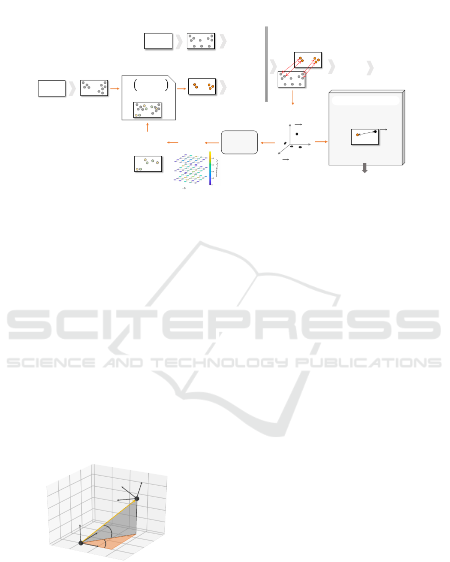
Figure 1: Block diagram of the APOFM method.

vious iterations. The technique employed for this pur-

pose is the Gaussian Process (GP) (Williams and Ras-

mussen, 2006). In Figure 1, all steps of this method

are shown.

In the ﬁrst iteration (t = 1), the relative pose is

estimated by solving the SVOM since all the projec-

tions of 3D scene points have the same probability

of being a correspondence. Therefore, the ﬁrst three

steps are to detect the feature points in each image (I

and I

), extract the descriptor vector of these points

and search correspondences according to a distance

measure between descriptors. The similarity measure

used for the binary feature descriptors is the Ham-

ming distance and the Squared Euclidean distance for

other description formats. This way, a set of 2D to 2D

correspondences has been obtained. from it, the next

step consists in estimating the relative motion through

the epipolar geometry. It corresponds to the two last

blocks in the diagram of Figure 1: essential matrix

and relative pose.

𝝓

𝜷

𝝆

𝐙

𝐭

𝐙

𝐭

𝟏

𝐘

𝐭

𝐗

𝐭

𝐗

𝐭

𝟏

𝐘

𝐭

𝟏

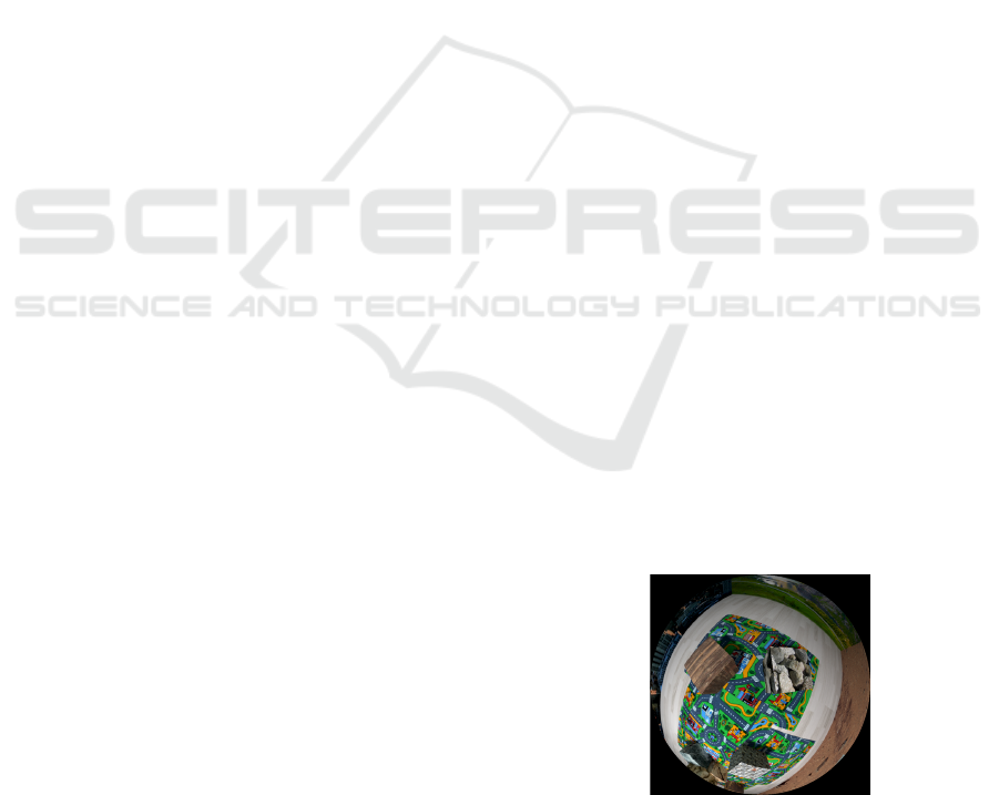
Figure 2: The relative translation expressed by two angles,

φ and β, and a scale factor ρ.

In this paper, the relative pose is expressed by ﬁve

angular parameters (θ, γ, α, φ, β) and a scale factor

(ρ). Three of the angular parameters are associated

with the orientation (θ, γ, α). The other two (φ, β),

along with the scale factor ρ are associated with the

translation expressed in spherical coordinates (Figure

2), where ρ is the relative distance between both cam-

era centers (except for a scale factor), φ is the polar

angle and β the elevation angle from the x-y plane. In

the experimental section, the values of these angular

parameters are estimated. At the end of this ﬁrst itera-

tion, the information about feature correspondences is

obtained. The steps considered by the APOFM to use

this information are explained in the following sub-

sections.

3.1 3D Probability Model

To create the model, ﬁrst, the 3D coordinates of each

pair of correspondences must be recovered, solving

the triangulation problem. In this sense, given a pair

of images, if the matching feature points are actually

the projection of the same 3D point, their rays must

intersect at this 3D point. However, this fact does not

always occur due to the presence of several types of

noise (e.g. error by non-precise calibration parame-

ters or noise during the feature detection). Therefore,

the triangulation problem is reduced to ﬁnding the

best solution, for instance, using the midpoint method

where the 3D point is assumed to be the midpoint of

the common perpendicular to both 3D lines.

However, the two 3D lines do not intersect in some

cases because the match of this pair of feature points

is a false positive, which means that they are not the

projection of the same 3D point though their descrip-

tor vectors are similar and therefore, they have been

wrongly associated during the matching search step.

To improve the SVOM regarding the false positives,

we have added a block, denominated false positive

ICINCO 2021 - 18th International Conference on Informatics in Control, Automation and Robotics

436

counter in the algorithm (see Figure 1), to evaluate

the effectiveness of the APOFM with respect to the

SVOM. In this block, given a 3D point

−→

whose

coordinates have been obtained with the pair of corre-

spondences (

−→

and

−→

t+1

), it is re-projected on the

second image

−→

using the camera model and if it is

near enough the feature point

−→

t+1

, it means that the

feature point is the projection of this 3D point and the

matched point is a true positive, otherwise it is a false

positive.

After solving the triangulation problem, the next

step to estimate the relative pose is to create the scene

model. To that end, the GP has been employed. The

GP block receives training input data that corresponds

to the set of 3D coordinates and training output data

that are a vector of ones indicating that the projec-

tion of these 3D points on the pair of images has been

considered as a matching point. Besides, there is a

set of test points that corresponds with the 3D points

that deﬁne the model. The output of the GP is the

mean and covariance of the predicted conditional dis-

tribution for the test points. The objective is to create

a probability model of the environment

−→

M j

, so this

prediction must take values between zero and one. To

that end, a logistic function (sigmoid) is employed.

Finally, the global map is updated using a Bayesian

Committee Machine (BCM).

3.2 Selecting Candidate Feature Points

Once the 3D scene model with probability is created

(t = 1) or updated (t > 1), the mobile robot moves

to a new position, and an image I

t+1

is taken. Then,

the feature points are detected. The next step con-

sists in projecting the 3D probability information on

this new image. To that end, both intrinsic and ex-

trinsic camera parameters must be known. The in-

trinsic ones have been previously obtained with the

calibration process. The extrinsic parameters are es-

timated by employing the vehicle model and apply-

ing the transformation from the mobile robot frame to

the camera frame (it is known since the camera is in-

stalled in the same position on board the mobile robot

at every moment). This odometry data is only used

for mapping from 2D to 3D points and from 3D to

2D.

At this stage of the algorithm, a two-set of

pixel points are obtained: one with image informa-

tion (feature points) and another with probability for

the search of correspondences (projection of the 3D

model scene). The selecting candidate features step

is given by a search for the nearest point in the sec-

ond set to each point in the ﬁrst set. This search is

based on a metric measure, concretely on the City-

Block and the technique to ﬁnd the nearest neighbor

is the Kd-tree algorithm.

A feature point will be considered as a candidate if

the calculated distance is lower than a speciﬁc thresh-

old (χ) whose value is given by the chi-square inverse

cumulative distribution function. If the feature point

is classiﬁed as a candidate to ﬁnd a matching in the

image I

, the probability of the nearest projected point

is associated with this feature point. The candidate

points can then be ﬁltered according to the probabil-

ity value associated, obtaining a set of candidate fea-

ture points whose probability to represent a matching

is higher than a minimum probability (ρ

min

The following steps correspond to the SVOM

(matching search, essential matrix and relative pose),

as explained for the ﬁrst iteration. However, the de-

scriptor vectors are only extracted from the candi-

date points since this is the set of features used in the

matching search.

4 EXPERIMENTS

As stated in Section 3, the APOFM method estimates

the relative pose from local feature points. Consider-

ing it, the experiments performed in this paper have

two main objectives: (a) evaluating the behaviour of

the APOFM with various local feature types to de-

termine which of them provides a more precise rela-

tive pose estimation; and (b) performing a comparison

between the APOFM and SVOM in order to assess

the improvement achieve with the APOFM method.

Therefore, a total of eight tests have been performed

as a result of the combination of the two methods and

the four local features: (1) SURF-SVOM, (2) SURF-

APOFM, (3) ORB-SVOM, (4) ORB-APOFM, (5)

FAST-SVOM, (6) FAST-APOFM, (7) KAZE-SVOM

and (8) KAZE-APOFM. In the ﬁgures, the results ob-

tained with SVOM are shown in orange colour and

with the APOFM method in grey colour.

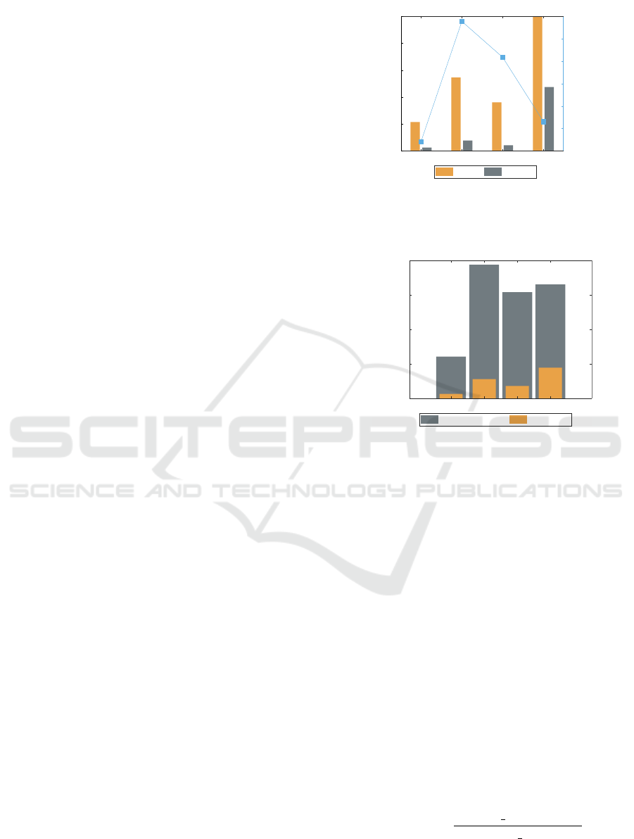
Figure 3: An example of ﬁsheye image available in the

dataset (Zhang et al., 2016).

To evaluate the inﬂuence of the kind of features,

we have carried out a study regarding the following

Evaluating the Inﬂuence of Feature Matching on the Performance of Visual Localization with Fisheye Images

437

aspects: the number of features detected with each lo-

cal feature and how many of them have been found as

a match on the other image (Section 4.1); the preci-

sion obtained in the matches search (Section 4.2); the

error during the estimation of the relative pose (Sec-

tion 4.3); and the computation time (Section 4.4). In

each ﬁgure, the result shown is the average of the val-

ues obtained with each pair of images. All experi-

ments have been carried out with a PC with a CPU

Intel Core i7-10700 R at 2.90GHz and Matlab as soft-

ware.

With respect to the images, we have used an open-

source and publicly available dataset (Zhang et al.,

2016). This dataset provides a set of ﬁsheye im-

ages model (see Figure 3), and an output ﬁle with the

camera positions where each image is taken (ground

truth). The camera followed a trajectory from which

the number of images taken is 200, with a resolution

of 640x480 pixels.

4.1 Number of Feature Points and

Matches Detected

As mentioned throughout this paper, both the SVOM

and the APOFM method solve the localization prob-

lem using local feature points detected on two images

and a set of correspondences between them. There-

fore, we will study it in this subsection.

First, Figure 4 shows the performance of the eight

combinations points/odometry method. The right ver-

tical axis of Figure 4 and the blue tendency show the

number of local feature points detected. Concerning

this, there is no distinction according to the odom-

etry method employed since the number of feature

points is independent of it, which means that it is the

same in both cases. The parameters of the features

have been chosen sin order to detect a high number

of points. Second, the number of these points that

ﬁnally have found their corresponding point on an-

other image is represented on the left axis of Figure

4. In this case, the number of matches depends on the

odometry method employed so, the number obtained

with each one is represented by a different bar. After

analyzing Figure 4, we can conclude that the highest

number of local feature points is obtained using ORB

and FAST. On the contrary, SURF provides the lowest

number of matches with both methods. In contrast,

when KAZE is employed, more feature points result

in matching points, although the number of points de-

tected on the image is not as elevated as using ORB or

FAST. As for the odometry methods, we can observe

that the SVOM algorithm ﬁnds more matches than

APOFM. This fact was expected in advance since the

second method does not use all the feature points de-

2000

3000

4000

5000

6000

7000

8000

Number of points

Matching

SURF ORB FAST KAZE

500

1000

1500

2000

2500

Number of matches

SVOM APOFM

Figure 4: The number of feature points detected is repre-

sented in the right axis, and the number of them that have

found a correspondence in the left axis.

Candidate points

SURF ORB FAST KAZE

2000

4000

6000

8000

num points

Features detected Candidates

Figure 5: APOFM method. The initial number of features

detected and number of them considered as matching can-

didates are shown to highlight how this method ﬁlters them

considering their probability of existence.

tected in this step, only those that have been consid-

ered as matching candidates due to their probability

of existence. Figure 5 is dedicated exclusively to the

APOFM method. It shows the number of features de-

tected, and how many of them have been considered

as matching candidates, this way, we can observe that

the matching search step using this method consid-

ers a lower number of feature points corresponding to

t+1

since the initial feature set has already been ﬁl-

tered by probability of existence.

4.2 Precision in the Matching Search

In addition to the study of the number of feature cor-

respondences, it is necessary to analyse how many of

these matchings are true positives or false positives.

To that purpose, the precision of the matching pro-

cess is calculated as:

Precision =

matches number − FP

matches number

(1)

where FP is the number of false positives, that is, pairs

of correspondences whose feature points are wrongly

ICINCO 2021 - 18th International Conference on Informatics in Control, Automation and Robotics

438

associated as the projection of the same 3D point. The

block added to the algorithm (false positive counter,

in Figure 1) returns this value. The precision is repre-

sented on the right axis of Figure 6 and the blue ten-

dency, and it is normalized from 0 to 1. The left axis

of Figure 6 shows, by means of bars, the ratio between

the number of feature points detected and the num-

ber of matches. The closer to one the precision value

is, the more accurate it is. Figure 6 shows that the

matching step using SURF is less accurate than using

the other local features. The precision difference is

considerable, taking into account that the precision in

the other features is higher than 0.99 and near to one

while in the case of SURF, it is lower than 0.98.

Ratio and precision

SURF ORB FAST KAZE

0.2

0.4

0.6

0.8

Matches/points

0.95

0.96

0.97

0.98

0.99

precision

SVOM APOFM

Figure 6: The ratio (left axis) and the precision (right axis)

during the matching search step.

4.3 Error Estimating the Relative Pose

The objective is to estimate the relative pose with the

highest accuracy. Therefore, the error must be stud-

ied to determine how a localization method performs

depending on the sort of feature points utilized as in-

put. In this subsection, the ﬁgures show, using bars,

the error of each odometry method with respect to the

ground truth.

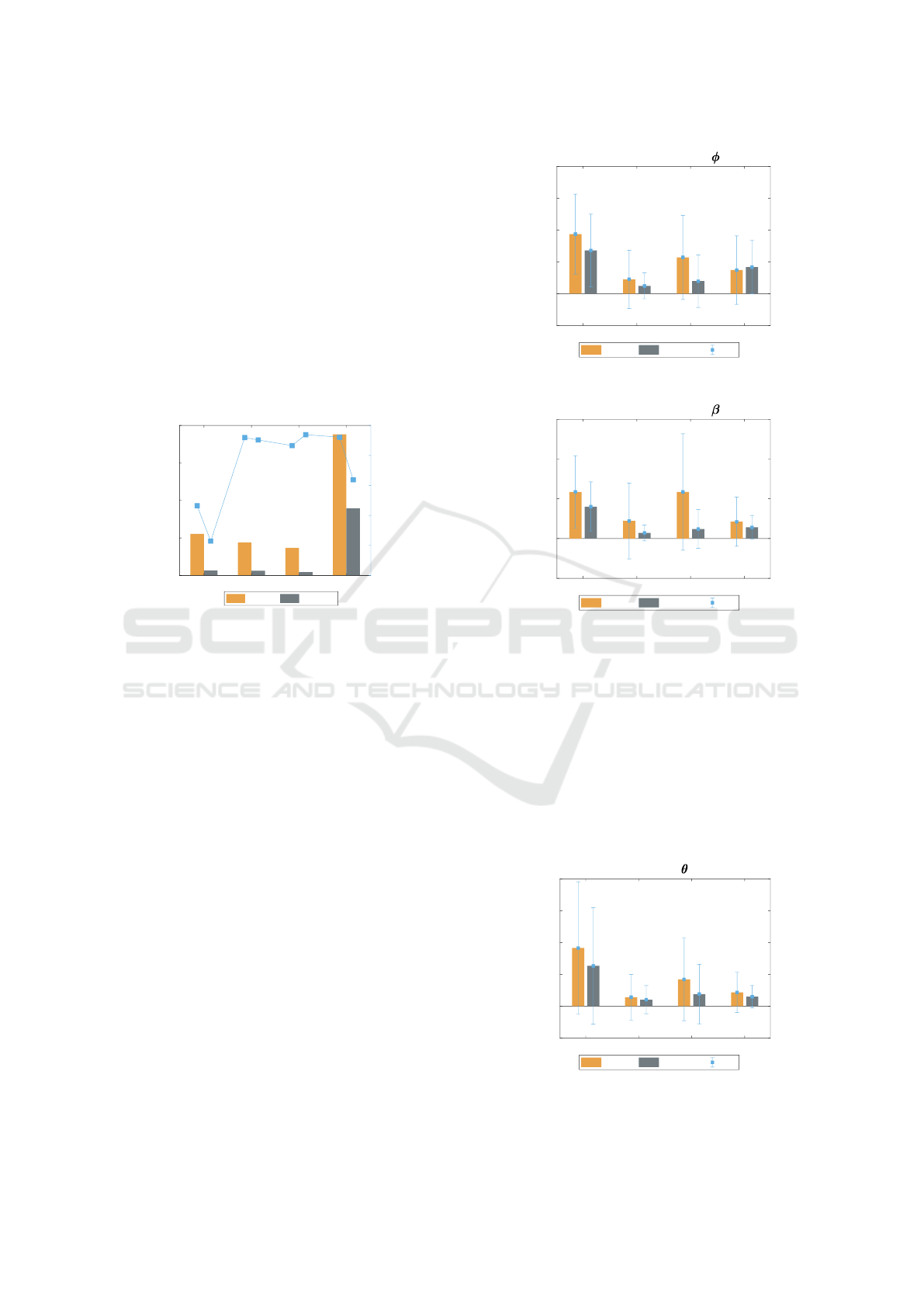
The errors estimating the relative translation are

represented in Figure 7 and Figure 8. The ﬁrst one is

related to the parameter φ, whereas the second ﬁgure

is associated with the parameter β. Analyzing both

ﬁgures, we can observe that the error is higher with

SURF. This fact was expected in advance due to its

worse precision commented in Section 4.2 and the

lowest number of points detected and matches. As

for the parameter φ (Figure 7), the APOFM method

presents a lower error with respect to SVOM in all

cases, except when using KAZE. However, there

is not a considerable error difference between both

methods in this case, though, concerning the standard

deviation, APOFM presents better results. The best

localization solution has been obtained with the com-

bination of the APOFM method and ORB, being the

Translation error

SURF ORB FAST KAZE

-20

angular error (

)

SVOM APOFM std

Figure 7: Error estimating the translation parameter φ.

Translation error

SURF ORB FAST KAZE

-20

angular error (

)

SVOM APOFM std

Figure 8: Error estimating the translation parameter β.

error in φ around 4

◦

. In contrast, the APOFM pro-

vides a lower error estimating the parameter β, inde-

pendently on the local feature type.

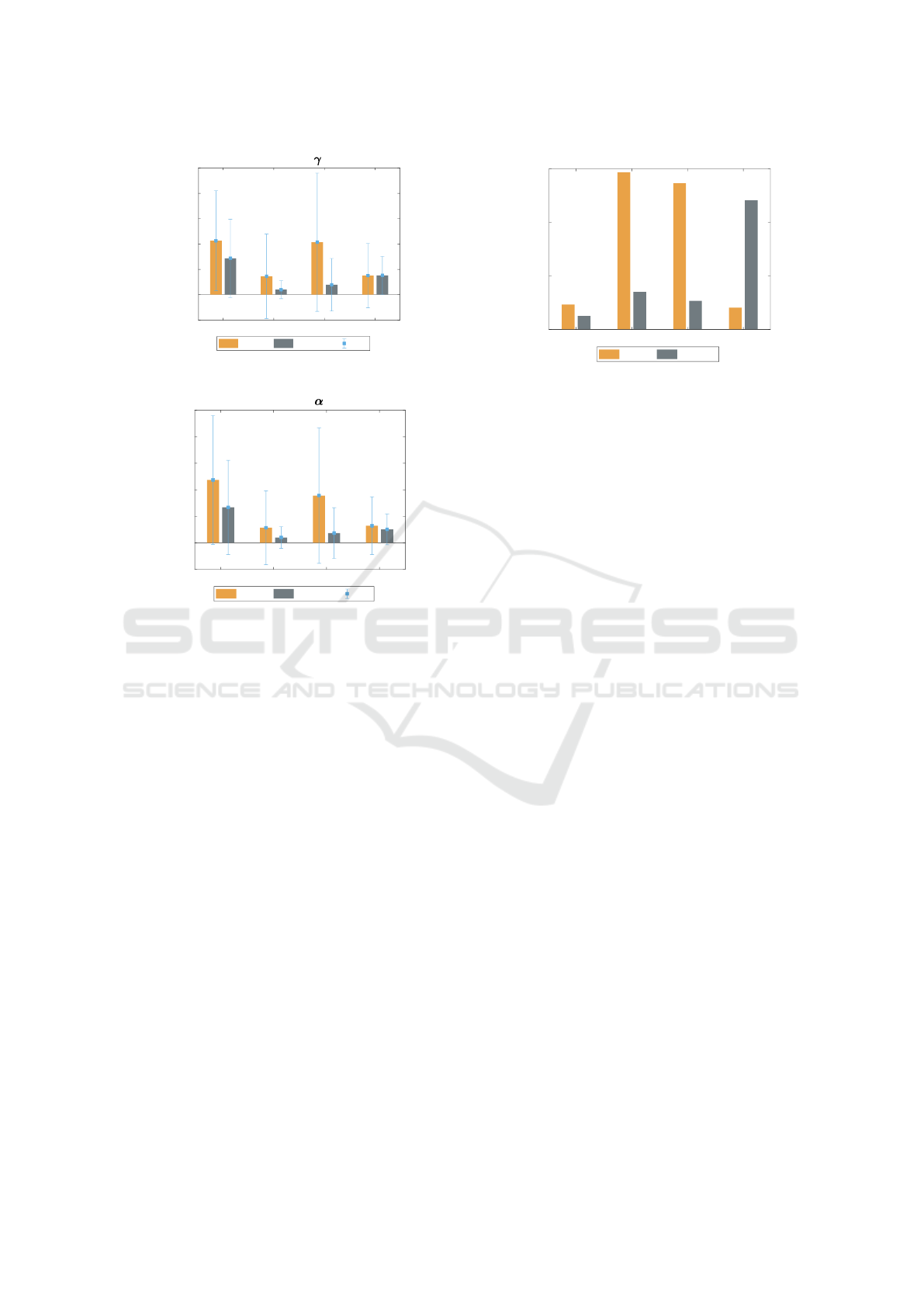
The relative orientation is expressed by three an-

gles (θ, γ and α), so Figure 9, Figure 10 and Figure

11 show the error estimating these parameters. As for

the method used, the APOFM estimates the orienta-

tion with more precision than SVOM. Similarly that

in the translation, the best localization solution, that

is, the one that provides lowest error, is obtained with

the ORB local feature.

Rotation error (Z-axis)

SURF ORB FAST KAZE

-0.2

0.2

0.4

0.6

0.8

angular error (

)

SVOM APOFM std

Figure 9: Error estimating the rotation parameter θ.

Evaluating the Inﬂuence of Feature Matching on the Performance of Visual Localization with Fisheye Images

439

Rotation error (Y-axis)

SURF ORB FAST KAZE

-0.5

0.5

1.5

2.5

angular error (

)

SVOM APOFM std

Figure 10: Error estimating the rotation parameter γ.

Rotation error (X-axis)

SURF ORB FAST KAZE

-0.5

0.5

1.5

2.5

angular error (

)

SVOM APOFM std

Figure 11: Error estimating the rotation parameter α.

4.4 Computation Time

Finally, it is also necessary to analyse the computation

efforts required by each of the combinations studied

in the previous subsections. Figure 12 compares the

computation times.

The time used during the relative pose estimation

is lower for the APOFM when the local features are

SURF, ORB and FAST. This is due to the fact that, in

the case of APOFM, the number of feature points cor-

responding to I

t+1

that have to ﬁnd a match is lower

than in the case of SVOM since the feature points

have been ﬁltered (candidates). This way, the time

associated with this step and the features SURF, ORB

and FAST is also lower, except when using KAZE.

5 CONCLUSIONS

In this paper, the information from the environment

is acquired by a ﬁsheye camera, and the localization

problem is solved using publicly available images.

We have studied the performance of our former

method (APFOM, (Valiente et al., 2018)) when differ-

ent sets of feature detectors and descriptors are con-

sidered as inputs. The APOFM characterizes the en-

Computation time

SURF ORB FAST KAZE

time (s)

SVOM APOFM

Figure 12: The computation time of each test is shown.

vironment by dynamically modelling 3D points with

certain probability of feature point existence. In this

manner, feature correspondences can be found in spe-

ciﬁc areas of the images. Such dynamic model is

obtained by an inference technique, the GP. In (Va-

liente et al., 2018), the authors evaluate this method

using images taken by a catadioptric vision system

and SURF features solely.

The present work has evaluated the behaviour of

the localization technique by means of an experimen-

tal setup consisting in: a total of eight tests accord-

ing to the combination of the method (the SVOM and

the APOFM) and the local feature type (SURF, ORB,

FAST and KAZE). For each one, we have studied sev-

eral aspects, such as the number of features detected

and matches; the precision regarding the correspon-

dences found and the pose estimation (by means of

the error made in each localization parameter), and

the time consumed to calculate the relative pose (con-

sidering all the steps of the algorithm).

From the analysis of the results, we can conclude

that the APOFM method has outperformed consider-

ably the SVOM with regards to the localization solu-

tion and the computation time when the local features

are SURF, ORB and FAST. The difference between

both methods when they use KAZE is slight, and the

error using the APOFM method is a little higher. The

combination of the APOFM method and ORB pro-

vides a more precise localization (the error is around

◦

for the translation parameter φ) besides a lower

computation time with respect to the SVOM.

In summary, the localization problem solved using

the APOFM method has been improved by employing

other feature point types, concretely ORB.

As future work, it will be interesting to evalu-

ate this method with other local feature points, such

as ASIFT (Yu and Morel, 2011), which is invariant

to afﬁne transformations. Moreover, another future

work will consider extending these comparative re-

sults to other non-linear image models.

ICINCO 2021 - 18th International Conference on Informatics in Control, Automation and Robotics

440

ACKNOWLEDGEMENTS

This work was supported in part by the Spanish

Government through the Project DPI 2016-78361-

R (AEI/FEDER, UE) ”Creaci

on de mapas mediante

etodos de apariencia visual para la navegaci

on de

robots”, and in part by the Generalitat Valenciana

through the Grant ACIF/2020/141 and the Project

AICO/2019/031 ”Creaci

on de modelos jer

arquicos y

localizaci

on robusta de robots m

oviles en entornos so-

ciales”.

REFERENCES

Alatise, M. B. and Hancke, G. P. (2020). A review on chal-

lenges of autonomous mobile robot and sensor fusion

methods. IEEE Access, 8:39830–39846.

Alcantarilla, P. F., Bartoli, A., and Davison, A. J. (2012).

KAZE features. In Fitzgibbon, A., Lazebnik, S., Per-

ona, P., Sato, Y., and Schmid, C., editors, Computer

Vision – ECCV 2012, pages 214–227, Berlin, Heidel-

berg. Springer Berlin Heidelberg.

Amor

os, F., Pay

a, L., Mayol-Cuevas, W., Jim

enez, L. M.,

and Reinoso, O. (2020). Holistic descriptors of om-

nidirectional color images and their performance in

estimation of position and orientation. IEEE Access,

8:81822–81848.

Aqel, M. O. A., Marhaban, M. H., Saripan, M. I., and Is-

mail, N. B. (2016). Review of visual odometry: types,

approaches, challenges, and applications. Springer-

Plus, 5(1):1897.

Bay, H., Ess, A., Tuytelaars, T., and Van Gool, L. (2008).

Speeded-Up Robust Features (SURF). Computer

Vision and Image Understanding, 110(3):346–359.

Similarity Matching in Computer Vision and Multi-

media.

Joshi, K. and Patel, M. I. (2020). Recent advances in lo-

cal feature detector and descriptor: a literature survey.

International Journal of Multimedia Information Re-

trieval, 9(4):231–247.

Matsuki, H., von Stumberg, L., Usenko, V., St

uckler, J.,

and Cremers, D. (2018). Omnidirectional DSO: Di-

rect Sparse Odometry With Fisheye Cameras. IEEE

Robotics and Automation Letters, 3(4):3693–3700.

Rom

an, V., Pay

a, L., Cebollada, S., and Reinoso,

O. (2020).

Creating incremental models of indoor environments

through omnidirectional imaging. Applied Sciences,

10(18).

Rosten, E. and Drummond, T. (2006). Machine learning

for high-speed corner detection. In Leonardis, A.,

Bischof, H., and Pinz, A., editors, Computer Vision

– ECCV 2006, pages 430–443, Berlin, Heidelberg.

Springer Berlin Heidelberg.

Rublee, E., Rabaud, V., Konolige, K., and Bradski, G.

(2011). ORB: An efﬁcient alternative to SIFT or

SURF. In 2011 International Conference on Com-

puter Vision, pages 2564–2571.

Scaramuzza, D. (2014). Omnidirectional Camera, pages

552–560. Springer US, Boston, MA.

Scaramuzza, D. and Fraundorfer, F. (2011). Visual odom-

etry [tutorial]. IEEE Robotics Automation Magazine,

18(4):80–92.

Tuytelaars, T. and Mikolajczyk, K. (2008). Local in-

variant feature detectors: A survey. Foundations

and Trends

 in Computer Graphics and Vision,

3(3):177–280.

Valiente, D., Pay

a, L., Jim

enez, L. M., Sebasti

an, J. M.,

and Reinoso,

O. (2018). Visual information fusion

through bayesian inference for adaptive probability-

oriented feature matching. Sensors, 18(7).

Valiente Garc

ıa, D., Fern

andez Rojo, L., Gil Aparicio, A.,

Pay

a Castell

o, L., and Reinoso Garc

ıa, O. (2012). Vi-

sual odometry through appearance-and feature-based

method with omnidirectional images. Journal of

Robotics, 2012.

Williams, C. K. and Rasmussen, C. E. (2006). Gaussian

processes for machine learning, volume 2. MIT press

Cambridge, MA.

Wirth, S., Carrasco, P. L. N., and Codina, G. O. (2013).

Visual odometry for autonomous underwater vehi-

cles. In 2013 MTS/IEEE OCEANS-Bergen, pages 1–6.

IEEE.

Yu, G. and Morel, J.-M. (2011). ASIFT: An Algorithm for

Fully Afﬁne Invariant Comparison. Image Processing

On Line, 1:11–38.

Zhang, Z., Rebecq, H., Forster, C., and Scaramuzza, D.

(2016). Beneﬁt of large ﬁeld-of-view cameras for vi-

sual odometry. In 2016 IEEE International Confer-

ence on Robotics and Automation (ICRA), pages 801–

808.

Evaluating the Inﬂuence of Feature Matching on the Performance of Visual Localization with Fisheye Images

441