Optimization-based Trajectory Prediction Enhanced with Goal

Evaluation for Omnidirectional Mobile Robots

Wei Luo

and Peter Eberhard

Institute of Engineering and Computational Mechanics,

University of Stuttgart, Pfaffenwaldring 9, 70569 Stuttgart, Germany

Keywords:

Goal Intention Evaluation, Monte-Carlo Sampling, Optimization, Trajectory Prediction, Complementary

Progress Constraint, Mobile Robot.

Abstract:

In this paper, an optimization-based trajectory prediction enhanced with goal evaluation for omnidirectional

mobile robots is proposed. The proposed approach tries to predict the mobile platform’s trajectory based on

its previous positions. A two-stage strategy is introduced. At the ﬁrst stage, the likely goal of the robot in the

scenario is evaluated based on an improved Bayesian framework, which also predicts the possible waypoints

in a discrete roadmap based on Monte-Carlo sampling in the future. Then, based on the predicted waypoints,

an optimization problem is formulated based on the complementary progress constraints, the system dynam-

ics, and the model constraints. After solving the proposed optimization problem, a more reasonable predicted

trajectory can be generated. At the end, an experimental scenario is set up, and it is veriﬁed with the experi-

mental data, whether the trajectories can be predicted well.

1 INTRODUCTION

Nowadays, robots are widely applied in different ap-

plications, such as logistic transport, industrial pro-

duction (Qian et al., 2017), and disaster relief (Su

et al., 2015). In most cases, the robots in the ﬁeld

are organized decentralized. Furthermore, in an en-

vironment with humans, the human beings’ potential

actions cannot be known to robots. Therefore, one of

the critical capabilities for these robots is the trajec-

tory prediction of the other robots or human beings

in the same working environment. Of course, such a

prediction assumes a reasonable ‘predictable’ behav-

ior and cannot consider sudden changes in the inten-

tion. One can increase the cooperation efﬁciency with

the predicted trajectory. For example, if the poten-

tial trajectory can be forecasted well, the navigation

method can consider this in the own motion planning

and avoid likely collisions. The collision probability

will be reduced once the trajectory of the other agents

can be predicted in advance. This ability is also inter-

esting in the application of autonomous systems, e.g.,

autonomous driving systems. The trajectory predic-

tion of the other vehicles and also the pedestrians on

https://orcid.org/0000-0003-4016-765X

https://orcid.org/0000-0003-1809-4407

the street can help autonomous cars to make a rea-

sonable decision and generate safer paths (Li et al.,

2019).

Let us describe the investigated scenario. A ﬂying

quadcopter is observing a scene with obstacles and

one or several robots on the ground and is recording

current position data for future use. The quadcopter

wants to approach one of the moving mobile robots

on the ground and for the purpose has to complete

and permanently update its own trajectory such that

at contact time the position and velocity of the quad-

copter and mobile ground robot agree. However, this

trajectory planning is not part of this paper. In this pa-

per it is considered, how the quadcopter predicts the

unknown but most likely path of the mobile ground

robot just based on information about its past mo-

tion. Of course, this has to assume that the mobile

ground robot behaviour in a ‘reasonable’ way and has

a certain intention which should be predicted. Nat-

urally, e.g., a pure random path would not follow an

intention and then no prediction would be possible.

When the quadcopter collects more and more infor-

mation about the mobile ground robots past motion

and where it approaches him, the prediction will be-

come more and more precise. Note that the quad-

copter can neither know the intention future path of

the mobile ground robot nor can it inﬂuence its mo-

Luo, W. and Eberhard, P.

Optimization-based Trajectory Prediction Enhanced with Goal Evaluation for Omnidirectional Mobile Robots.

DOI: 10.5220/0010551802630273

In Proceedings of the 18th International Conference on Informatics in Control, Automation and Robotics (ICINCO 2021), pages 263-273

ISBN: 978-989-758-522-7

263

tion or trajectory planning. The trajectory planning

for the mobile ground robot computed on the quad-

copter only serves the purpose to make the best, most

likely prediction. The scenario is very similar to the

one described in (Best and Fitch, 2015), difference

will be commented later. Technically, we introduce

a two-stage trajectory prediction strategy for omni-

directional mobile robots, only utilizing the previous

observable robot positions in a known environment.

The proposed approach tries to identify the movement

intention of the observed mobile robot, and predicts

its potential trajectory within the reasonable time al-

location, see Fig. 1.

x [m]

y [m]

Figure 1: Trajectory prediction based on the previous robot

positions marked with red circles in a known environment.

The grey squares are the predicted path waypoints, which

are based on the sampling results from the shaded traces.

The ﬁnal predicted most likely trajectory is connected by

blue circles.

The proposed strategy consists of an improved

goal evaluation-based Bayesian framework and an

optimization-based trajectory generator. At the ﬁrst

stage, the proposed framework evaluates the likely

goal of the observed robot in the known environ-

ment and creates a cursory path, which is only com-

posed of several key waypoints that have a relatively

high inferential probability. At the second stage,

given the estimated most likely path waypoints, an

optimization-based framework is formulated based

on the complementary progress constraints (CPC),

which handles the progress over the predicted way-

points, and the model constraints that are observed in

the past positions. Then, the optimization framework

is applied for generating a reasonable trajectory pre-

diction for the omnidirectional mobile robot.

Our main contributions for the proposed two-stage

trajectory prediction strategy are:

• An improved goal evaluation-based Bayesian path

waypoint predictor is introduced, which uses only

the previous robot positions, and guesses the

likely motion. A momentum parameter is uti-

lized, which signiﬁcantly improves the efﬁciency

of the trajectory sampling. Furthermore, a motion

tendency-based goal intention probability func-

tion is applied for evaluating the robot’s potential

goal according to its recent positions.

• Instead of using a velocity distribution to predict

the trajectory of the observed robot along the lin-

ear sample paths in the map graph in (Best and

Fitch, 2015), here an optimization-based solution

is proposed, to guess an optimized path with a rea-

sonable time-allocation passing through the esti-

mated waypoints under the observable robot con-

straints based on CPC.

The paper is organized as follows. Section 2 gives

an overview of the state-of-the-art in related works.

In Section 3, the proposed two-stage approach is de-

scribed. Finally, the experimental results are illus-

trated in Section 4, and conclusions are presented in

Section 5.

2 RELATED WORK

Trajectory Model-based Method. Trajectory

model-based approaches utilize some pre-deﬁned

model assumptions to assist the prediction of the

possible poses of the observed agent in the future.

In (Acuna et al., 2018), the observed agent’s tra-

jectory was assumed as being polynomial, and the

observer only needs to ﬁnd a ﬁtting parameter set

for the polynomial trajectory based on the previous

trace of the observed agent. In (Sch

oller et al., 2020),

the research showed that even a constant velocity

model could make a good prediction of the pedestrian

motion compared with state-of-the-art approaches.

Neural Network-based Method. With the rapid

development of neural network technology, several

researchers utilized neural networks to predict the se-

quential trajectory of the observed agent. One of

the typical network structures, recurrent neural net-

works (RNN), exhibit the ability to handle time se-

ries problems with data-driven techniques. The long

short-term memory (LSTM), which is a variation of

RNN, was utilized to predict the trajectory of vehi-

cles on the street in (Dai et al., 2019). Some ap-

proaches used generative models to predict the trajec-

tory. In (Gupta et al., 2018), the generative adversar-

ial networks (GANs) were ﬁrst successfully applied

ICINCO 2021 - 18th International Conference on Informatics in Control, Automation and Robotics

264

to predict a course of the pedestrian with a recurrent

sequence-to-sequence model.

Goal-Conditional-based Method. In some recent

works, instead of directly predicting the trajectory of

the observed agent, the procedure of the prediction is

divided into two or multiple stages. At the ﬁrst stage,

the goal of the observed agent will be evaluated, and

then the trajectory will be predicted based on the past

data and the evaluated goal. In (Best and Fitch, 2015),

a Bayesian mathematical formulation is used to esti-

mate the agent’s intention, and the resulting probabil-

ity distribution was used to generate the trajectory in

the future. In (Dendorfer et al., 2020) the goal con-

dition was combined with the GANs, the proposed

method showed a better performance than the typical

generative models. However, the physical limitations

of the observed agent are ignored, and the predicted

trajectory is lack of time information in these works.

3 APPROACH

The task of this paper is to predict the future trajec-

tory of the omnidirectional robot on the 2D ground

plane. Note that a trajectory in this work is deﬁned

as a path combined with a corresponding time alloca-

tion. The past trajectory is available from measure-

ments, and will be utilized as input of the proposed

algorithm of this work. At each time step t

, the pro-

posed algorithm will predict a sequence of the om-

nidirectional robot positions marked with X

i+1:i+k

i+ j

= (x

i+ j

) ∈ R

|j = 1, ..., k} ∈ X for the

next time points t

i+1

,. .. ,t

i+k

given the past observa-

tion set X

1:i

, where X denotes the continuous space

of the whole scenario.

3.1 Goal Evaluation-based Bayesian

Path Waypoint Prediction

At the ﬁrst stage of the proposed approach, based on

the already stored trajectory, the potential goal of the

observed robot is evaluated based on the goal inten-

tion evaluation, and the future potential path is esti-

mated based on the Bayesian framework. The process

of this stage is shown in Algorithm 1.

3.1.1 Goal Intention Evaluation

The proposed method in this work focuses on pre-

dicting a likely trajectory for the robot with a certain

destination in the known environment. Although the

exact goal of the observed robot cannot be known in

advance, we assume that the set of all potential goal

Algorithm 1: Bayesian Goal Evaluation-based Path Way-

point Prediction Approach.

1: // pre-computation

2: /∗ generate roadmap based on k-PRM* ∗/

3: DB(·,·),

X ← k-PRM*(X ,n

nodes

)

4: // main while loop

5: while mission in process do

6: /∗ get the current robot position from sensor

and ﬁnd the closed vertex in roadmap

X ∗/

← x

8: /∗ goal intention update∗/

9: Pr(θ

1:i

) ← Eq. 1

10: /∗ trajectory waypoint prediction ∗/

11: the counting map M

(θ

x, j) ∈ R

×c

×k

12: for each θ

∈ Θ do

13: N

← N ×Pr(θ

1:i

)

14: for each n ∈ N

15:

i+1:i+k

← MC-sampling(

,θ

)

16: end for

17: for each j ∈[1,k] do

18: /∗ sum-pooling ∗/

19:

← Pooling(

∈

i+1:i+k

)

20: M

(

x, j) = M

(

x, j) + 1

21: end for

22: end for

23: /∗ waypoint generation∗/

24: for each θ

∈ Θ do

25: for each j ∈[1,k] do

26: x

pred

← argmax

M(θ

η,max

x, j)

27: end for

28: end for

29: end while

regions Θ := {θ

|η ∈[1,.. ., n

]}is feasible and ﬁnite,

where the number of goal regions is deﬁned as n

. For

instance, a potential goal could be the exit of the sce-

nario, the working station, or the shelves in logistics

warehouses, etc.

In this work, we use the probability distribution

to describe the intention of the mobile robot to each

goal region. Then, a motion tendency-based goal in-

tention probability function is introduced, which only

takes the l latest robot positions to evaluate the robot’s

motion intention. In each step, given the new coming

observation x

, the goal intention can be estimated by

Pr(θ

1:i

) ∝

∏

j=i−l

(exp( f

j−1

,θ

) − f

,θ

))

·( f

j−1

,θ

) + 1)),

(1)

where the function f

indicates the shortest path dis-

tance between two given positions, and the function f

describes the cosine of the angle between three given

Optimization-based Trajectory Prediction Enhanced with Goal Evaluation for Omnidirectional Mobile Robots

265

positions in 2D, which is deﬁned as

a,b

b,c

c) =

b −a

a) ·(c

c −b

b −a

akkc

c −b

. (2)

First, the proposed goal intention function evaluates

the path distance changes to every evaluating goal re-

gion θ

observing the l latest robot positions. The

target could be deemed to be the most likely goal of

the robot, if its path distances to the robot in the last

l positions are most reduced. Additionally, the goal

region which is located behind the direction of mo-

tion should have a lower probability of being selected.

Hence, a component with the cosine of the angle be-

tween the previous robot motion direction and the po-

tential motion direction from the robot’s current posi-

tion to a candidate goal region is multiplied.

3.1.2 Discrete Roadmap

Instead of working on the continuous 2D space, which

has inﬁnite possible states to describe the mobile

robot, we utilize a discrete roadmap

X at the ﬁrst

stage to represent the robot’s position and the po-

tential path between the its current position and the

goal region. The discrete roadmap is a graph data

structure, which is composed of several randomly dis-

tributed nodes and the edges that represent collision-

free paths between nodes. The total number of nodes

nodes

on the roadmap should be speciﬁed balancing

the computational time and the coverage rate by the

user. The paths through the roadmap are utilized

to approximate the potential route of the observed

robot. Besides, based on the nodes and the edges

on the roadmap, the shortest path between two arbi-

trary nodes is determined by the A* algorithm. In this

work, the k-nearest optimal probabilistic roadmap (k-

PRM*) is utilized to create an ofﬂine roadmap (Kara-

man and Frazzoli, 2011).

PRM

√

6(A

free-space

/π)

0.5

+ 1)

(log(n

nodes

)/n

nodes

)

0.5

PRM

=2elog(n

nodes

(3)

where the free area of the scenario is marked with

free-space

. To improve the real-time computing per-

formance, the shortest paths between nodes and their

corresponding path distances will be calculated of-

ﬂine and stored in the database DB(a

a,b

b), where the

nodes a

a and b

b are two arbitrary nodes on the roadmap.

3.1.3 Improved Probabilistic Dynamics Model

To determine the next position x

i+1

based on its prob-

ability distribution, a probabilistic dynamic model is

introduced given the previous position x

and the goal

region. Instead of only considering the path distance

as in (Best and Fitch, 2015), the probabilistic dynamic

model in this work introduces a new parameter β to

demonstrate the effect of the linear momentum on the

probability distribution. The improved probabilistic

dynamics model is deﬁned as

Pr(x

i+1

,θ

) ∝

exp(−α( f

i+1

) + f

i+1

,θ

) − f

,θ

)))β.

(4)

Note that it is unnecessary to estimate the probability

for every node on the roadmap, and one only needs

to consider the nodes in the area

∈

X that can be

reached within next time step, see Fig. 2.

i−1

i−2

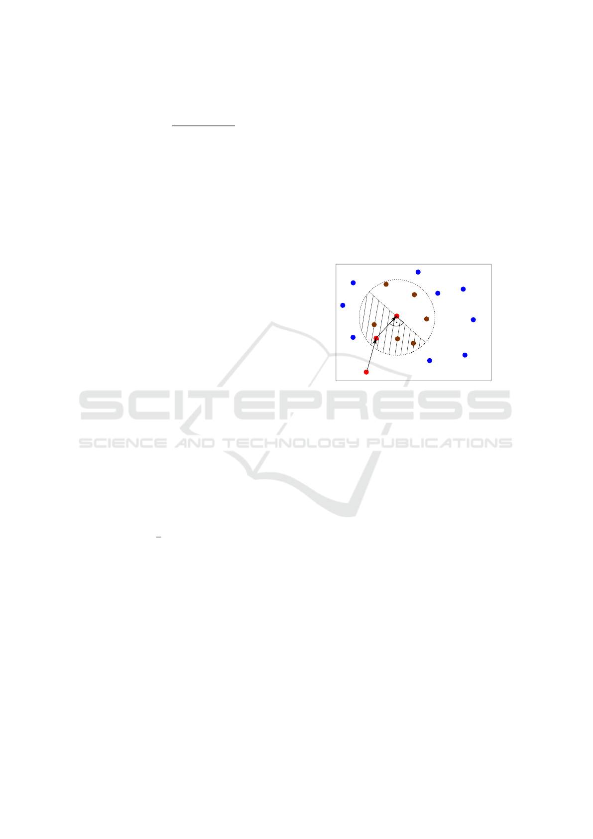
Figure 2: Illustration for the probabilistic dynamic model.

The dotted circle illustrates the candidate area

, and the

nodes, that the robot can arrive within next time step, are

marked with brown circles. On the contrary, nodes which

are out of range, are marked with blue circles.

In Eq. 4, the parameter α is non-negative and

needs to be speciﬁed by the user. When α → 0, the

probability for each node in

will be almost iden-

tical when the effect of parameter β is ignored. On

the contrary, if α → +∞, the assumption is that the

robot always takes the shortest path to the goal posi-

tion. However, the choice of the parameter α could

be tricky since it is challenging to balance the explo-

ration and the exploitation when only considering the

distance relationship with parameter α, especially for

the scenarios with multiple goal regions. Therefore,

the linear momentum parameter β is introduced

β = max{1e−6, f

i−1

i+1

)kx

−x

i−1

k}.

(5)

In Eq. 5, if a candidate

i+1

in next step has a re-

markable moving direction difference compared with

the last observed motion, the result of the momentum

parameter will be set close to zero, which dominates

the candidate’s probability of being chosen. For in-

stance, given the past course X

i−2:i

marked with red

circles in Fig. 2, the candidates, which are located in

the shadow region, are less likely to be chosen as the

potential path waypoint of the mobile robot, based on

the proposed probabilistic dynamics model in Eq. 4.

ICINCO 2021 - 18th International Conference on Informatics in Control, Automation and Robotics

266

3.1.4 Bayesian Path Waypoint Prediction

Based on the improved probabilistic dynamic model

in Eq. 4 and the goal intention evaluation from Eq. 1,

one can estimate the next possible position

i+1

∈

considering a candidate goal region through

Pr(x

i+1

1:i

,θ

) = Pr(x

i+1

,θ

) ×Pr(θ

1:i

(6)

Intuitively, one can further, based on Eq. 6, recur-

sively estimate the position of the robot x

i+ j

in the

coming time horizon

Pr(x

i+ j+1

1:i

,θ

) =

∑

i+ j

∈

i+ j

[Pr(x

i+ j+1

i+ j

,θ

)

×Pr(x

i+ j

1:i

,θ

)].

(7)

However, as mention in (Best and Fitch, 2015), the

analytical evaluation of Eq. 7 is difﬁcult due to the

branching factor of the roadmap. Therefore, the

trajectory waypoints will be estimated through the

Monte-Carlo sampling approach.

Based on the evaluated goal intention probability

distribution in Eq. 1, N

trajectories will be sampled

from current position x

to the goal region θ

. In

each sampling, the next possible position node

i+ j

in the region

i+ j−1

is chosen based on the probabil-

ity given the improved probabilistic dynamic model

in Eq. 4.

Rather than greedily choosing the most sampled

nodes at each prediction time step, a sum-pooling pro-

cedure in this work is utilized to generate the ﬁnal

predicted waypoints. Each visited node in

i+1:i+ j

at the time step j will be pooled and converted into

a grid graph

X ∈ R

×c

, where the parameters c

and c

are the number of grids in x-/y-coordinate of

X , respectively. Then, for each goal region, the vis-

iting times of each grid on the graph will be summed

into a counting map M

at each prediction time step,

which indicates the grid’s frequency of being visited.

The sum-pooling process sacriﬁces the prediction ac-

curacy to reduce the distribution unbalance of the gen-

erated nodes on the roadmap

X and eliminate the

prediction of too short paths, especially when a rel-

atively small α in Eq. 4 is chosen. At the end, for

each goal region, the most visited grid to the goal re-

gion at each prediction time step will be recorded and

formulated as the predicted waypoint of the observed

robot as X

pred

i+1:i+k

:= {x

pred

i+ j

∈ R

|j ∈ [1, ...,k ], θ

3.2 Optimization-based Trajectory

Prediction

The proposed method in Section 3.1 can effectively

provide a rough path based on the goal intention eval-

uation and Monte-Carlo sampling approach. How-

ever, the predicted path is discontinuous and only

composed of several key waypoints. Besides, the def-

inition of the available area

is based on the param-

eters r

PRM

and k

PRM

in Eq. 3. These two parameters

concern the probabilistic completeness of the gener-

ated roadmap, and the physical limitations of the ob-

served robot are neglected. Therefore, the time step

mentioned in last section cannot provide a precious

time allocation of the predicted paths. At the second

stage, instead of using a velocity model to estimate

the time allocation along the predicted line segments

in (Best and Fitch, 2015), an optimization-based tra-

jectory prediction in this work is proposed to predict a

more reasonable trajectory in the future based on the

previously indicated path waypoints.

The proposed optimization formulation will deter-

mine an optimized trajectory that fulﬁls several rea-

sonable constraints. First, the robot’s dynamics func-

tion and some observable physical limitations need to

be satisﬁed. For instance, the observed maximal ab-

solute velocity and the acceleration can be estimated

given the robot’s previous trajectory, and they are uti-

lized to bound the predicted state of the mobile robot

in the optimization problem. Besides, since the robot

has its certain motion intention, the robot is unlikely

to linger about the scenario. Therefore, the estimated

total travel time and the optimized trajectory distance

should be minimized as possible. Furthermore, the

predicted trajectory should pass through the previ-

ously estimated path waypoints in sequence. To that

end, the complementary progress constraints (CPC)

are introduced in the proposed optimization problem,

which will be detailed in the next section.

3.2.1 Complementary Progress Constraints

At this stage, an optimized trajectory with a ﬁxed

time interval will be generated to present the most

likely trajectory of the observed omnidirectional mo-

bile robots in the future. The time interval dt is de-

ﬁned as t

, where the number of the new gen-

erated optimized trajectory nodes is marked as n

and t

is the total travel time of the optimized tra-

jectory. To handle the predicted path waypoints, a

progress variable set Λ

Λ := {λ

∈R

|p = [1,..., n

]}

is introduced to indicate whether the optimized tra-

jectory passes through the desired waypoints in a se-

quence (Foehn and Scaramuzza, 2020). Here, n

the number of path waypoints estimated from last sec-

tion, which satisﬁes n

> n

obviously. Due to the

sum-pooling procedure in last section, the number of

the waypoints n

meets n

≤ k , since the predicted

waypoint at different time step j may stay at the same

grid on the counting map M

Optimization-based Trajectory Prediction Enhanced with Goal Evaluation for Omnidirectional Mobile Robots

267

The progress variable λ

in Λ

Λ indicates the re-

lationship between the w-th waypoint x

pred

and the

optimized trajectory node

at the time step p. If

has passed through the given the waypoint x

pred

the progress variable λ

will become zero; other-

wise it will keep its inertial value. To ensure the op-

timized trajectory passes through the predicted path

waypoints in order, the following condition should be

fulﬁlled

≤ λ

w+1

, ∀w ∈ [1,n

−1] and p ∈ [1,n

], (8)

which ensures the optimized

passes the waypoint

pred

earlier than the next waypoint x

pred

w+1

. Besides,

each element λ

is initialized as one at the begin-

ning of the optimization, and it has the following basic

characters further:







0 ≤ λ

≤ 1

= 1 ∀w ∈ [1,n

] and p ∈ [1,n

]

= 0

. (9)

Instead of introducing a new progress change pa-

rameter in (Foehn and Scaramuzza, 2020) to handle

the state switch of the progress variable that may in-

crease the burden of solving the optimization prob-

lem, the complementary progress constraints (CPC)

in this work are formulated as

prog

pred

,Λ

Λ)

=[(λ

−λ

p+1

)

| {z }

( f

pred

) −ν

)

| {z }

]

= 0,

(10)

where the function f

estimates the Euclidean distance

between two given positions. Furthermore, it is not a

wise strategy to force the optimized trajectory

X pass-

ing all the predicted waypoints X

pred

i+1:i+k

exactly. On

the one hand, the predicted waypoints may have some

outliers, which will strongly impact the result of the

optimized trajectory. On the other hand, the accuracy

of the predicted waypoints is limited by the grid size

) from last stage. Therefore, in Eq. 10, a relax-

ation parameter ν

is introduced, which satisﬁes

0 ≤ ν

≤ d

tolerance

,∀p ∈ [1,n

−1], (11)

where d

tolerance

indicates the maximum acceptable

offset to the predicted waypoint. The complemen-

tary progress constraint deﬁned in Eq. 10 consists of

two components, P

and P

. If an optimized trajec-

tory waypoint

gets closed enough to one of the

predicted waypoint x

pred

, which satisﬁes the area de-

ﬁned in Eq. 11, the component P

will become zero.

In this case, the next progress variable λ

p+1

for the

same waypoint can be reduced to zero to meet the

constraint deﬁnitions in Eq. 9. Otherwise, the com-

ponent P

should always stay zero to meet the com-

plementary constraint in Eq. 10.

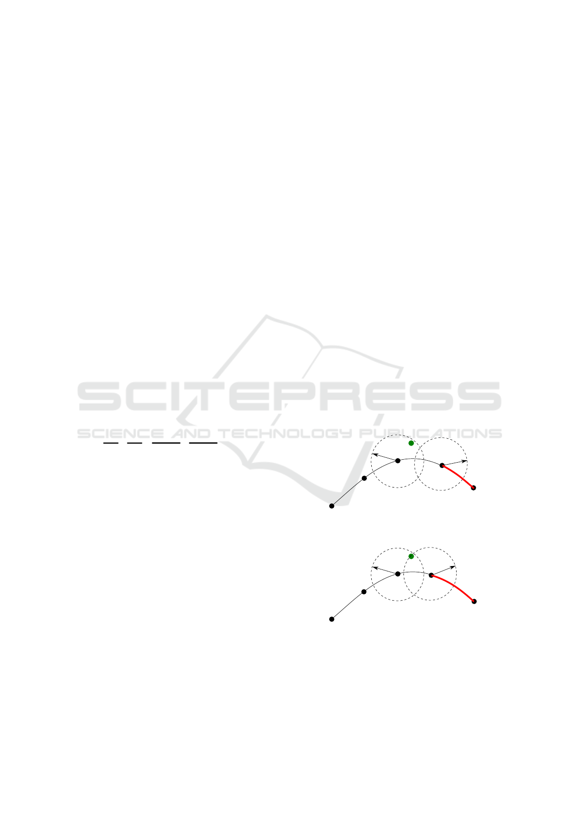
Ideally, a predicted path waypoint should attract

only one optimized trajectory waypoint. For instance,

in Fig. 3a, once an optimized trajectory waypoint

fulﬁlls the tolerance condition to the predicted

path waypoint x

pred

, the rest progress variables λ

4:n

should go to zeros. However, the constraint deﬁned in

Eq. 10 alone cannot prevent a non-optimal trajectory

waypoint distribution, see Fig. 3b. Since the posi-

tion of the

fulﬁlls all constraints in Eqs. 10-11, the

progress variable λ

has not been restrained at all. In

this case, a predicted path waypoint could attract more

than one optimized trajectory waypoints, which may

result in an unbalance waypoint distribution. Further-

more, the unbalance waypoint distribution may cause

an inappropriate estimation of the total travel time.

Since the proposed optimized trajectory has a ﬁxed

time interval, the total travel time is depended on the

maximum track length between every two adjacent

optimized trajectory waypoints and the physical lim-

itations of the observed robot. If a non-ideal way-

point distribution occurs, an unexpected long trajec-

tory track may be predicted, which results in an un-

necessary long total travel time. To prevent the non-

ideal distribution, the sum of all process variables will

be minimized in the proposed optimization formula-

tion.

= 1

pred

= 1

= 0

(a) An ideal waypoint distribution.

= 1

pred

= 1

0 ≤ λ

≤ 1

= 0

(b) A non-ideal waypoint distribution.

Figure 3: Illustration for different waypoint distributions

with the progress variables. Under the non-ideal way-

point distribution, the trajectory track between

and

in Fig. 3b is longer than the one in Fig. 3a, which may lead

to errors in the total travel time estimation.

ICINCO 2021 - 18th International Conference on Informatics in Control, Automation and Robotics

268

3.2.2 Optimization Formulation

To implement the optimization formulation for the

trajectory prediction, the state of the mobile robot and

its dynamics will be deﬁned ﬁrst. Note that, in this

work an omnidirectional mobile robot is utilized as

the observed target; however, the proposed approach

also can be applied to other robots, for which one

should just specify the appropriate state deﬁnition and

dynamic limitations accordingly.

The state of the omnidirectional mobile robot is

described as

x := [ ˘x, ˘y,

˘x,

˘y]

, and the control input for

the robot is assumed to be

u := [F,φ]

, where F is the

unknown applied control force on the omnidirectional

mobile robot, and the angle between the applied force

and the x-axis of the global system is deﬁned as φ.

Although we cannot know the robot’s exact mass, we

still can assume that the input force is mass normal-

ized, which is proportional to the robot acceleration.

Therefore, the dynamic of the omnidirectional mobile

robot can be described as

dyn



˙x, ˙y,F cos(φ), F sin(φ)



. (12)

The full optimization state set of the optimization

problem X

opt

consists of the robot states

and the

control inputs

of the robot, the progress parameter

and the relaxation parameter ν

at every time step

p. Besides, the total travel time t

is also introduced

as one of the optimization states.

The cost function of this optimization problem is

composed of three components. First, the total travel

time should be short under some observable physi-

cal limitations. Then, the total traveled trajectory dis-

tance is to be minimized, which makes optimizer pre-

fer a non-aggressive trajectory given the same total

travel time. The third component is the sum of all

progress variables, which prevents the non-ideal way-

point distribution. Based on the introduction above,

the optimization problem is formulated as

min

opt

+ γ

−1

∑

l=1

(k˘x

l+1

− ˘x

, ˘y

l+1

− ˘y

)

+ γ

∑

p=1

∑

w=1

s.t.

dt = t

= x

p+1

+ dt f

RK4

(

),∀p ∈ [1,n

−1]

min

≤

≤ x

max

,∀p ∈ [1,n

]

min

≤

≤ u

max

,∀p ∈ [1,n

−1]

and further constraints based on Eqs. 8 −11,

(13)

where f

RK4

is the 4th-order Runge-Kutta approxima-

tion of the system dynamic from Eq. 12, and the

parameters γ

1/2/3

determine the weights of the to-

tal travel time, the trajectory length and the sum of

the progress variable set, respectively. Furthermore,

the constraints of the control input u

max,min

, and the

system state x

max,min

can be determined relying on

the previous robot positions. By implementing of

the optimization problem, CasADi (Andersson et al.,

2019) is utilized with the solver IPOPT (W

achter and

Biegler, 2005).

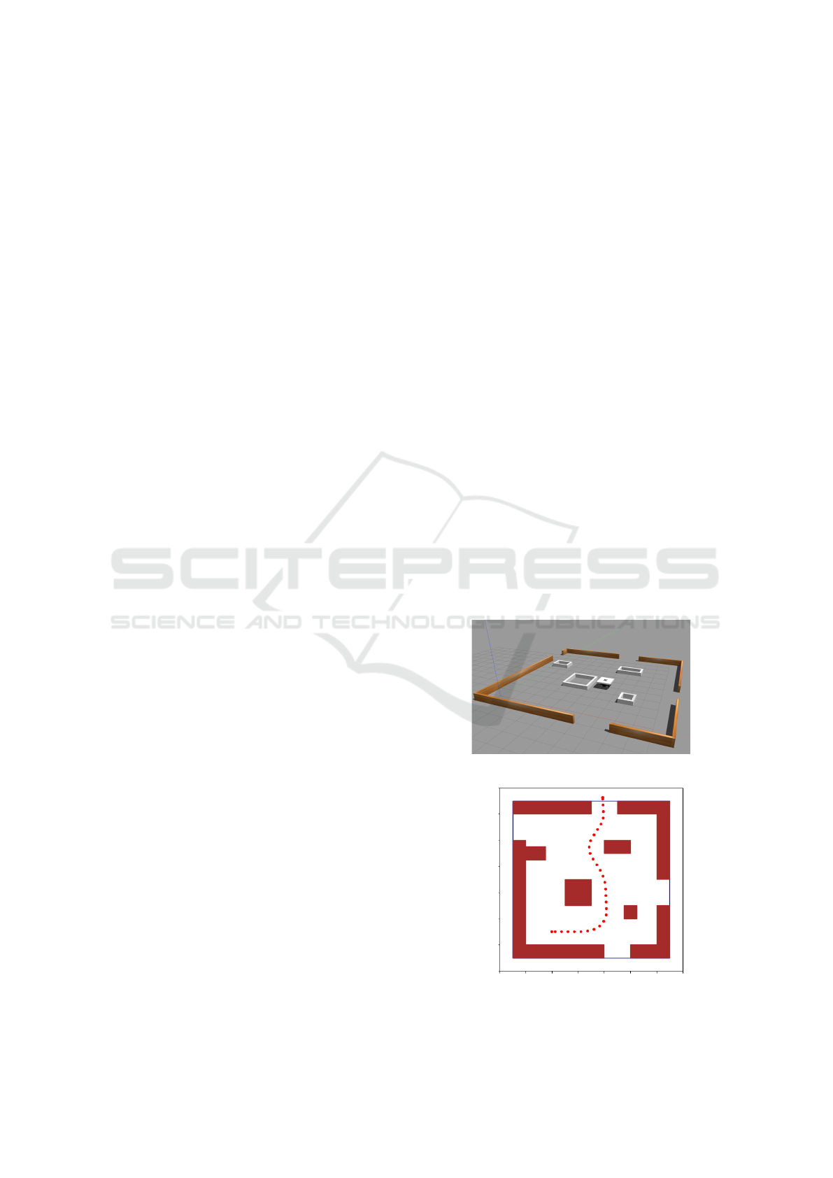
4 EXPERIMENTAL VALIDATION

To verify the performance of the proposed two-stage

approach in this work, a scenario is set up in the sim-

ulation platform Gazebo, where the blocks indicate

the obstacles which the omnidirectional mobile robot

will avoid, see Fig. 4. In the simulation experiment,

total of 500 nodes are randomly generated to create a

k-PRM

∗

roadmap. Among them, 469 nodes present

the possible positions of the omnidirectional mobile

robot, and the rest nodes are randomly distributed in

the goal regions. So, there are 14539 path connections

in total, and the path between each node and its travel

distance are estimated ofﬂine. The whole ofﬂine pro-

cedure is processed on a machine with Intel i9 CPU,

and the calculation time is less than 5.7 seconds.

Figure 4: An experimental simulated scenario in Gazebo.

x [m]

y [m]



-2

-2 0 2 4 10 128

Figure 5: Previously unknown path of the mobile robot.

Optimization-based Trajectory Prediction Enhanced with Goal Evaluation for Omnidirectional Mobile Robots

269

0.34

0.03

0.22

0.41

(a) Sampling at t

0.36

0.53

0.09

0.02

(b) Sampling at t

0.59

0.41

0.0

0.89

0.10

0.01

0.0

(d) Sampling at t

0.34

0.03

0.22

0.41

(e) Waypoints at t

0.36

0.53

0.09

0.02

(f) Waypoints at t

0.59

0.41

0.0

(g) Waypoints at t

0.89

0.10

0.01

0.0

(h) Waypoints at t

Figure 6: Path waypoint prediction at stage one. Figures 6a- 6d illustrate all predicted paths for the next k = 8 prediction steps

at the given simulation time step. The corresponded path waypoint estimations are shown in Fig. 6e- 6h.

4.1 Path Waypoint Prediction

In the experiment, the omnidirectional mobile robot

goes to the goal region



while avoiding the obsta-

cles in the scenario. The ground truth trajectory of

the mobile robot is marked with red circles, which are

sampled by 1 Hz, as illustrated in Fig. 5.

In each step, the newly measured pose of the robot

will be taken, and the potential path waypoints in the

future will be evaluated based on Algorithm 1. In this

experiment, 8 time steps (k = 8) in the future will be

estimated, and in each iteration, N = 200 samplings

will be processed. The calculation time for the path

waypoint prediction in each iteration requires 0.04

seconds on average using the Numba library (Lam

et al., 2015).

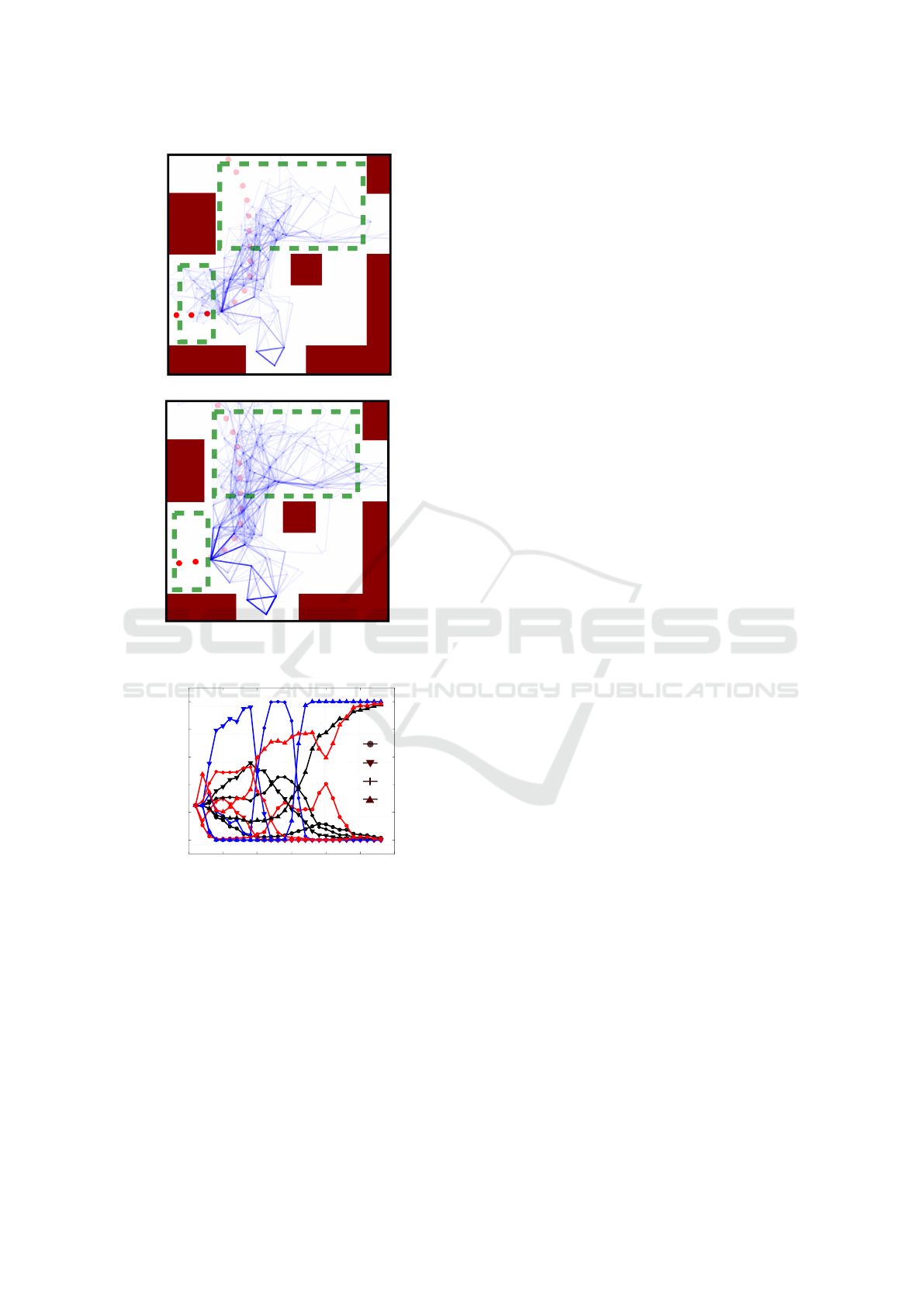
In Fig. 6, the predicted path waypoints at four

different simulation time steps are illustrated. Fig-

ures 6a-6d show the sampled paths in the next eight

time steps in the future based on the Monte-Carlo

sampling method. By utilizing the proposed prob-

abilistic dynamics model, the sampling efﬁciency

is improved signiﬁcantly. In Fig. 7, the proposed

method is compared with the model in (Best and

Fitch, 2015) under same sampling conditions (N =

200, α = 1.5). The proposed model has more con-

centration on sampling the nodes in front of motion

direction due to the linear momentum parameter in

Eq. 5, instead of wasting the sampling with the nodes

behind the current motion tendency, especially on the

areas marked in Fig. 7. Based on the sampling results,

the predicted path waypoints at given simulation time

steps are illustrated in Figs. 6e-6h, respectively. Note

that only the predicted paths to the goal region with

a goal intention over 30% will be drawn. The ﬁnally

predicted path waypoints after the sum-pooling pro-

cedure are illustrated with grey squares.

During the experiment, the evaluated goal in-

tention changes for all four goal regions are illus-

trated in Fig. 8. The proposed goal intention model

is compared with the model in (Best and Fitch, 2015)

with two different parameter α setups. As expected,

the estimated intentions based on the model in (Best

and Fitch, 2015) are highly depended on the choice

of parameter α. If the parameter α is set to a large

value, the evaluated goal intention will increase or

decrease drastically. On the contrary, the model will

become unresponsive given a small value of α. The

proposed goal intention evaluation function provides

a relatively stable performance and it can response to

the robot moving tendency ﬂeetly. For instance, be-

tween the simulation steps t

and t

, the robot may

tend to move in the upper-left direction, see Figs. 6c

and 6g. In theory, given previous robot positions, both

region



and region



should have a similar goal in-

tension to the observed robot during this time. How-

ever, compared with the model from (Best and Fitch,

2015), only the proposed model shows a signiﬁcant

response to the potential change of robot’s intention.

ICINCO 2021 - 18th International Conference on Informatics in Control, Automation and Robotics

270

(a) Model in (Best and Fitch, 2015).

(b) Proposed model.

Figure 7: Sampling efﬁciency comparison.

20 25 30

simulation time step

0.0

0.2

0.4

0.6

0.8

1.0

probability



Figure 8: Evaluated goal intention changes during the ex-

periment. The result of the proposed goal intention func-

tion in red is compared with the intention inference model

in (Best and Fitch, 2015) with α = 0.5/5.0, which are

marked with black and blue, respectively.

4.2 Trajectory Estimation

Once the path waypoints are predicted, the guessed

future trajectory of the omnidirectional mobile robot

will be estimated by solving the proposed optimiza-

tion approach. Each trajectory estimation can be ac-

complished within 0.24 seconds. To quantitatively

verifying the performance, only the predicted trajec-

tories to the goal region



are taken in the compar-

ison. In Fig. 9, the predicted trajectories at four dif-

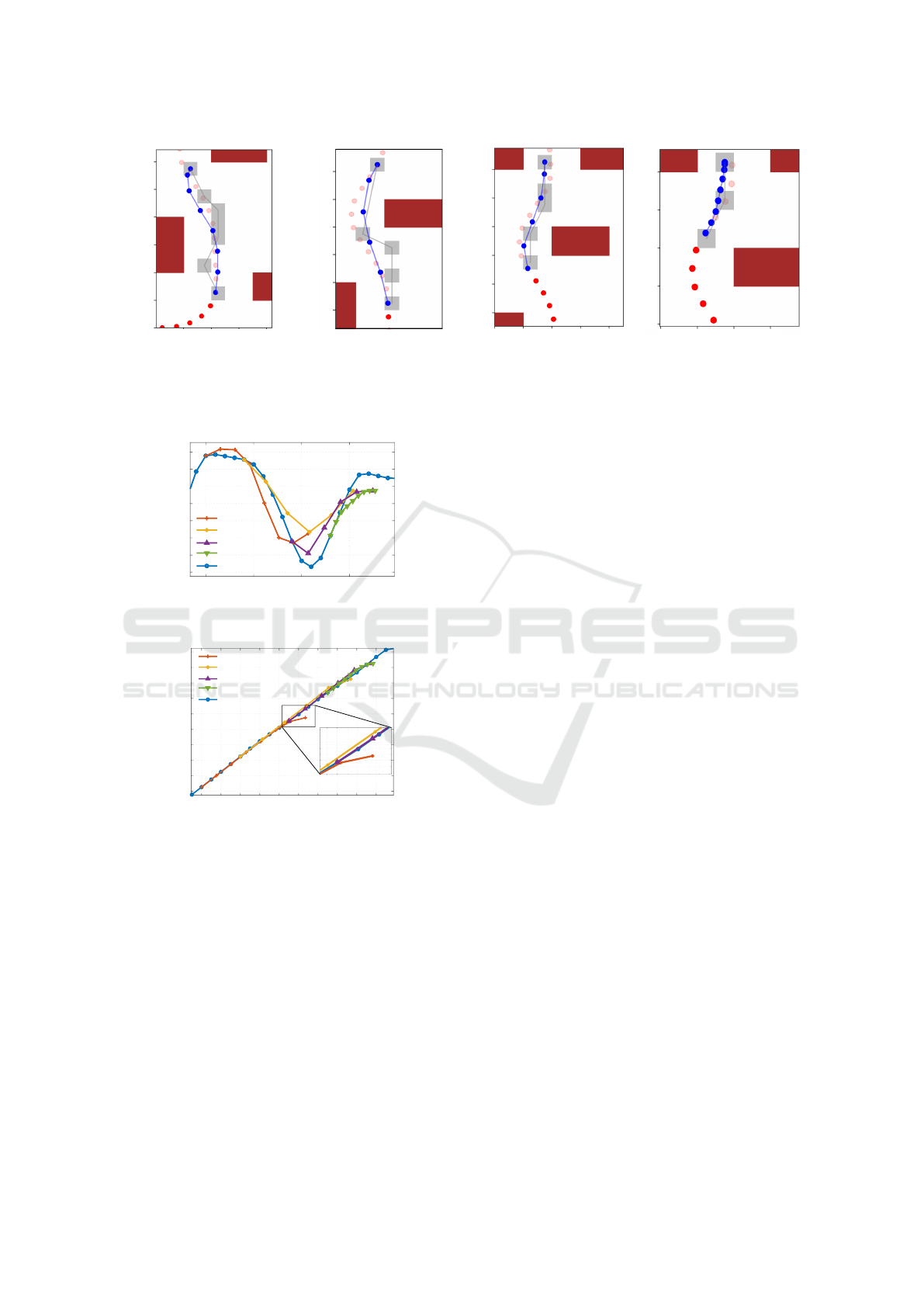
ferent simulation time steps are presented. Although,

the future ground-truth trajectory marked with pink

circles is not yet known, the proposed method can es-

timate the potential trajectory based on the sampling

results, which does not stay far away from the ground-

truth trajectory. Besides, compared with the predicted

path waypoints, the predicted trajectories are smooth

and continuous, which are more reasonable for the

mobile robots.

A further advantage of solving the proposed opti-

mization problem is that one obtains not only the pre-

dicted trajectory in the future, but also the total travel

time t

of the predicted trajectory. Compared with the

vague time step deﬁnition for the predicted path way-

points, the optimized trajectory has a ﬁxed time in-

terval between each predicted robot positions. There-

fore, every optimized trajectory waypoint has its own

estimated arrival time, which is essential for the ap-

plications, such as navigation planning and the colli-

sion avoidance. In Fig. 10, the predicted trajectories

at different simulation time steps (t

, t

and t

)

are compared with the ground truth trajectory of the

mobile robot. The results on both coordinates show a

good prediction, and the maximal error along the pre-

diction time horizon is less than 0.5 m. Considering

the grid size of the counting map and the optimiza-

tion constraint d

tolerance

that both are set to 0.5 m, the

predicted results are acceptable.

5 CONCLUSION

In this paper, a novel two-stage strategy is proposed

for predicting the potential trajectory of an omnidi-

rectional mobile robot given its past trajectory. The

effectiveness and efﬁciency of the proposed strategy

are veriﬁed in the simulation experiment. The results

show that the proposed method can identify goal in-

tentions of the observed robot based on its latest posi-

tions, and the errors of the ﬁnally predicted trajectory

and its allocated time stay in the acceptable range. In

future work, one may consider applying the proposed

algorithm to hardware experiments in more scenarios.

ACKNOWLEDGEMENTS

This research is funded by the German Research

Foundation (DFG) under Germany’s Excellence

Strategy - EXC 2075 - 390740016, project PN4-

4 “Theoretical Guarantees for Predictive Control in

Optimization-based Trajectory Prediction Enhanced with Goal Evaluation for Omnidirectional Mobile Robots

271

x [m]

y [m]

(a) Predicted trajectory at t

x [m]

y [m]

(b) Predicted trajectory at t

x [m]

y [m]

x [m]

y [m]

(d) Predicted trajectory at t

Figure 9: Results of the optimization-based trajectory prediction. The grey squares are the predicted path waypoints. The

ﬁnal predicted trajectory is marked with blue circles.

ground truth

20 25 30

simulation time step

4.8

5.2

5.6

6.0

6.2

5.8

5.4

5.0

x [m]

(a) Predicted results on the x axis.

ground truth

simulation time step

2.0

6.0

10.0

8.0

4.0

18 26 30

y [m]

19 20

6.4

7.0

7.6

(b) Predicted results on the y axis.

Figure 10: The optimized trajectory prediction results at the

iteration time step t

10/14/19/23

Adaptive Multi-Agent Scenarios”. Also, this research

beneﬁted from the support by the China Scholarship

Council (CSC, No. 201808080061) for Wei Luo.

REFERENCES

Acuna, R., Zhang, D., and Willert, V. (2018). Vision-

based uav landing on a moving platform in gps de-

nied environments using motion prediction. In Latin

American Robotic Symposium, Brazilian Symposium

on Robotics (SBR) and Workshop on Robotics in Edu-

cation (WRE), pages 515–521, Joao Pessoa, Brazil.

Andersson, J. A. E., Gillis, J., Horn, G., Rawlings, J. B., and

Diehl, M. (2019). CasADi – A software framework

for nonlinear optimization and optimal control. Math-

ematical Programming Computation, 11(1):1–36.

Best, G. and Fitch, R. (2015). Bayesian intention inference

for trajectory prediction with an unknown goal des-

tination. In IEEE/RSJ International Conference on

Intelligent Robots and Systems (IROS), pages 5817–

5823, Hamburg, Germany.

Dai, S., Li, L., and Li, Z. (2019). Modeling vehicle interac-

tions via modiﬁed lstm models for trajectory predic-

tion. IEEE Access, 7:38287–38296.

Dendorfer, P., O

sep, A., and Leal-Taix

e, L. (2020). Goal-

GAN: Multimodal trajectory prediction based on goal

position estimation. In Asian Conference on Com-

puter Vision (ACCV), pages 1–17, virtual conference.

Foehn, P. and Scaramuzza, D. (2020). CPC: Complemen-

tary progress constraints for time-optimal quadrotor

trajectories. In Robotics: Science and Systems, pages

1–12, virtual conference.

Gupta, A., Johnson, J., Li, F.-F., Savarese, S., and Alahi, A.

(2018). Social GAN: Socially acceptable trajectories

with generative adversarial networks. In IEEE Con-

ference on Computer Vision and Pattern Recognition

(CVPR), pages 2255–2264, Salt Lake City, USA.

Karaman, S. and Frazzoli, E. (2011). Sampling-based algo-

rithms for optimal motion planning. The International

Journal of Robotics Research, 30(7):846–894.

Lam, S. K., Pitrou, A., and Seibert, S. (2015). Numba: A

LLVM-based python JIT compiler. In Proceedings of

the Second Workshop on the LLVM Compiler Infra-

structure in HPC, pages 1–6, New York, USA.

Li, J., Ma, H., and Tomizuka, M. (2019). Conditional gener-

ative neural system for probabilistic trajectory predic-

tion. In IEEE/RSJ International Conference on Intel-

ligent Robots and Systems (IROS), pages 6150–6156,

Macao, China.

Qian, J., Zi, B., Wang, D., Ma, Y., and Zhang, D. (2017).

The design and development of an omni-directional

mobile robot oriented to an intelligent manufacturing

system. Sensors, 17(9):1–15.

Sch

oller, C., Aravantinos, V., Lay, F., and Knoll, A. (2020).

ICINCO 2021 - 18th International Conference on Informatics in Control, Automation and Robotics

272

What the constant velocity model can teach us about

pedestrian motion prediction. Robotics and Automa-

tion Letters (RA-L), 5(2):1696–1703.

Su, X., Zhang, M., and Bai, Q. (2015). A wireless mo-

bile robots deployment approach for maximising the

coverage of important locations in disaster rescues. In

IEEE/WIC/ACM International Conference on Web In-

telligence and Intelligent Agent Technology (WI-IAT),

volume 2, pages 17–20, Singapore.

achter, A. and Biegler, L. T. (2005). On the implemen-

tation of an interior-point ﬁlter line-search algorithm

for large-scale nonlinear programming. Mathematical

Programming, 106(1):25–57.

Optimization-based Trajectory Prediction Enhanced with Goal Evaluation for Omnidirectional Mobile Robots

273