Numerical Investigation of the Lateral Dynamic

Behaviour of the Anaconda

Python Kabeya Tshibamba

, Guyh Dituba Ngoma

and Fouad Erchiqui

University of Kinshasa, Department of Mechanical Engineering, Kinshasa, Democratic Republic of the Congo

University of Quebec in Abitibi-Témiscamingue, School of Engineering’s Department, 445, Boulevard de l’Université,

Rouyn-Noranda, Quebec, J9X 5E4, Canada

Keywords: Single Track Vehicle, Multibody System, Lateral Dynamic, Linear Stability, Eigenmodes, EasyDyn.

Abstract: This paper deals with the study of a particular single track vehicle, named Anaconda. Numerical simulations

are performed to assess the vehicle’s linear dynamic behavior. Indeed, multibody models of each component

of the Anaconda and the one of the entire vehicle are developed and linearized around stationary states. The

out-of-plane linearized sub-models are then used to have more insight in the lateral behaviour of the Anaconda

and the influence of one of its component, the pedal module, on this behaviour is outlined. These tasks are

carried out within the EasyDyn framework, an open source multibody library. Informative observations on

the simulation results help to find out some features of the Anaconda concerning its linear dynamic behaviour;

and some comment are made on the possibility of controlling its unstable eigenmodes.

1 INTRODUCTION

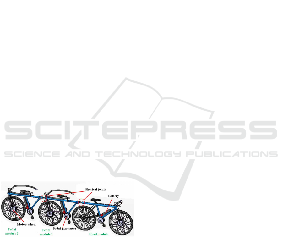
Anaconda is an in-line polycycle with reference to

single track vehicles, like bicycle and motorcycle. It

is composed of a head module which is a classical

bicycle followed by some pedal modules as shown in

Fig. 1.

Figure 1: Anaconda with two pedal modules.

This vehicle can transport several people one on

each module. Modules are connected each other by

spherical joints, and each pedal module is equipped

with a rear steered wheel so as its rider can contribute

in the vehicle balance and help in the following the

prescribed path; while the rider on the head module

decide which path to follow.

In this conceptual model, electric generators

provide energy when riders pedal. This energy is

managed by a central unit in order to redistribute it in

a proper manner to motor-wheels and store the

exceeded energy in batteries (Verlinden and Kabeya,

2012; Kabeya and Verlinden, 2010).

Anaconda as bicycles are human-powered

vehicles and nowadays the latter are used as healthy

and less pollutant transportation means. Riding a

bicycle can be learned intuitively and, when

mastered, this activity becomes a second nature.

However, the dynamic behaviour behind the

bicycle riding is more complex. The modularity of the

Anaconda makes its dynamic behaviour much more

complex than that of the bicycle and its investigation

is a challenging task.

The main issues in studying single track vehicle

are their stability characteristics and their dynamic

behaviour; and literature contains papers outlining

their dynamic studies (Sharp, 1985; Sharp, 1971;

Limebeer and Sharp 1971; Cossalter, 2006, Meijaard

et al., 2007).

This paper is concerned with the stability of an

Anaconda composed of one pedal module. Thanks to

the well established stability analysis of single track

vehicle, the aim of this study is to describe the lateral

stability of the Anaconda and to figure out the

influence of the pedal module. Numerical simulations

are carried out on multibody models of the vehicles;

based on the EasyDyn framework. Models concerned

in this study are those of the head module alone, the

Kabeya Tshibamba, P., Dituba Ngoma, G. and Erchiqui, F.

Numerical Investigation of the Lateral Dynamic Behaviour of the Anaconda.

DOI: 10.5220/0010551403190326

In Proceedings of the 11th International Conference on Simulation and Modeling Methodologies, Technologies and Applications (SIMULTECH 2021), pages 319-326

ISBN: 978-989-758-528-9

319

pedal module alone and an Anaconda with one pedal

module. Simulation results allow us to get more

insight in the lateral stability features of this vehicle

and to figure out the pedal module influences.

2 EasyDyn FRAMEWORK AND

VEHICLE’S MODELS

2.1 EasyDyn Framework

The studied mechanical models are developed

according to a multibody approach influenced by

EasyDyn (Verlinden et al., 2005; Verlinden et al.,

2013).

EasyDyn is C++, open source and flexible,

multibody library from the Department of the

Theoretically Mechanics, Dynamics and Vibrations

of the Faculty of Engineering of the University of

Mons in Belgium.

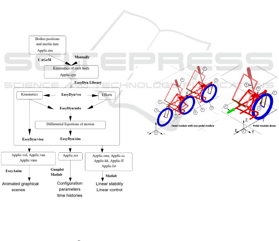
EasyDyn uses minimal coordinates to describe the

kinematics of rigid bodies connected by joints, thanks

Figure 2: EasyDyn simulation data flow.

to homogeneous transformation matrices; and the

principle of virtual power to derive the equations of

motion which are then integrated according to the

Newmark scheme (Newmark-





). Fig. 2 depicts the

simulation data flow in the EasyDyn framework.

The process starts with a Mupad file (Applic.mu)

which contains bodies’ inertia data and their relative

configurations expressed in term of the vehicle

configuration parameters. A symbolic tool called

CAGeM is used to generate symbolically the

kinematics of the vehicle. The resulted C++ file

(Applic.cpp) from CAGeM contains basic EasyDyn

command lines; and the user can include in this file

other EasyDyn command lines dedicated to his

application. Among the output files of this process

there are those required for the stability analysis of

the multibody systems under this research.

2.2 Mechanical Model

The Anaconda mechanical model was presented in

(Verlinden and Kabeya, 2012); where a multibody

approach was used by taking into account the

confirmed modelling assumptions made for single

track vehicle: bodies are considered to be rigid,

rider’s lower body is firmly attached to the module

frame, rider’s upper body can rotate about the

longitudinal axis of the module frame, tire-ground

contact is modelled as force element.

Fig. 3 illustrates the mechanical models of an

Anaconda composed of a head module with one pedal

module and a pedal module alone.

Figure 3: Riders-vehicle mechanical model.

The number of bodies (n

) and the one of degrees

of freedom (n

) of each system are summarized in

Tabs. 1 and 2. Parameters defining these degrees of

freedom are considered as configuration parameters.

Three vehicle’s models are investigated in this

work:

 The head module alone: n

= 6, n

= 10;

 The pedal module alone: n

= 6, n

= 6;

 The Anaconda with one pedal module: n

= 10,

= 16.

SIMULTECH 2021 - 11th International Conference on Simulation and Modeling Methodologies, Technologies and Applications

320

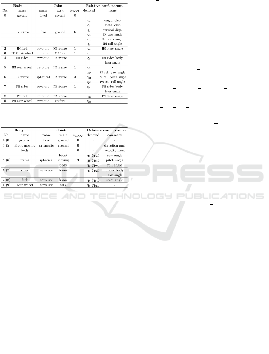
Table 1: Bodies and their relative degrees of freedom for

the Anaconda with one pedal module.

Table 2: Bodies and their relative degrees of freedom for

the pedal module alone.

Taking advantages of the parametric and generic

model of the Anaconda implemented in EasyDyn

(Kabeya and Verlinden, 2011), the numerical model

of the head module alone and the one of the Anaconda

with one pedal module are derived from the same

mechanical model.

The implementation of the pedal module alone is

made apart from the mechanical model presented in

Fig. 3. The pedal module is considered as a trailer

towed by a front moving body, replacing the head

module, whose motion is imposed. Physically, this

corresponds to the hypothesis that the head module

motion is not affected by the one of the pedal module.

2.3 Mathematical Model

For each vehicle’s model, the n

second order

equations of motion are derived and recasted in a

matrix form as:

M(q

) . q



+ h(q,q



) = g(q,q



,t)

(1)

where:

 q

is a (n

,1) vector gathering all the

configuration parameters;

 M is a (n

) mass matrix;

 h

is a (n

,1) vector gathering contributions of

centrifugal and Coriolis forces;

 g

is a (n

,1) vector gathering contributions of

external forces.

The forces taken into account in these models are

gravity and tyre-ground contact forces.

Furthermore, equations of motion are linearized

around a stationary state, defined as the state in which

the vehicle is let going straight ahead in a constant

configuration position q



and at a constant forward

velocity. The linearized equations are given as:

M . Δq



+ CT . 𝚫q + KT . 𝚫q = 0

(2)

where:

 Δq

= q – q



is the relative configuration

parameter vector defined with respect the

stationary state position q



;

 CT is a (n

) tangent damping matrix;

 KT is a (n

) tangent stiffness matrix.

For the linearization state, the lateral or out-of-

plan dynamic is decoupled from the in-plane one

(Koenen, 1983). Then sub matrices concerned with

out-of-plane dynamic: the reduced mass matrix (M



the reduced tangent damping (C



) and the reduced

tangent stiffness matrix (K



) are drawn from their

respective counterparts of the entire linearized system

by taking into account only the concerned

configuration parameters ( q



). The configuration

parameters involved in the out-of-plane dynamic are:

 The lateral displacement, the yaw, roll and steer

angles for the head module alone: n

= 4;

 The yaw, roll and steer angles for the pedal

module alone: n

= 3;

 The combination of the above two

configuration parameters for an Anaconda with

one pedal module: n

= 7.

Moreover, it is to highlight that rider’s upper body

degree of freedom is frozen in these models. This

configuration parameter together with the rider’s legs

are involved in the human control activities

attempting to maintain the vehicle balance. Their

influence where proved to be less significant with

respect to the steer angle (Kooijman et al., 2009).

The out-of-plane matrices are recasted in an

equivalent state space model:

 = A . x

(3)

where:

 x

is the reduced state vector of dimension (n

,1)

with n

= 2*n

; and is equal to

Numerical Investigation of the Lateral Dynamic Behaviour of the Anaconda

321

x = 



q



 (4)

 A is the evolution matrix of dimension (n

)

defined from the reduced matrices as:

A = 

−(M



)





−(M



)







(5)

with 0 and I the zero and identity matrices of

appropriate dimensions.

The evolution matrix is used in the sequel for the

computation of eigenvalues and eigenmodes of the

vehicle’s out-of-plane dynamic. Positions of

eigenvalues in the complex plane will vary with the

forward speed. The stability analysis of eigenmodes

is rely on these positions.

3 SIMULATION RESULTS

3.1 Modes Determination Procedure

For each vehicle, simulations are made as follows:

 The vehicle is brought in a steady state

condition letting it run straight ahead at a

constant velocity. The velocity ranges from 0.2

to 10 m/s with a step of 0.1 m/s are selected;

 The linearization of the equations of motion is

performed around this steady state

configuration;

 The text files containing the matrices of the

linearized equations of motion from EasyDyn

are retrieved under Matlab where the subset of

the lateral dynamics is extracted and recasted in

an equivalent state space model.

 Eigenvalues are computed for each forward

velocity and their evolution analysed.

The two first step are performed with EasyDyn.

Combination of the information from eigenvalues

evolution over the forward speed, mode shapes and

their animations are used to distinguish them from

each other.

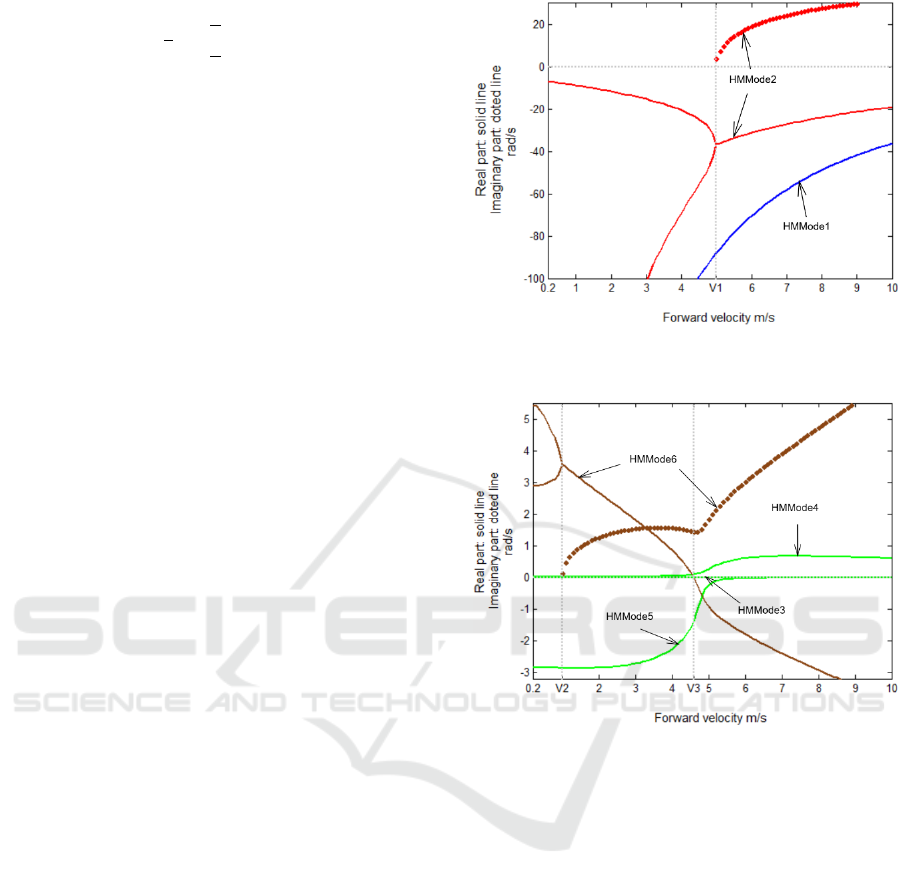
3.2 Modes of the Head Module Alone

According to the considered mechanical model, six

distinct head module’s modes are observed from the

eight eigenvalues computed. They are denoted from

HMMode1 to HMMode6. Evolutions of their

eigenvalues over the forward speed are given in Figs.

4 and 5.

Figure 4: HM modes evolution over the forward speed

range (HMMode1 and HMMode2).

Figure 5: HM modes evolution over the forward speed

range (HMMode3, HMMode4, HMMode5 and

HMMode6).

HMMode1, 2, 3 and 5 are stable modes whereas

HMMod4 and 6 are unstable ones. HMMode6

evolves to the stable region as the forward speed

increases with a crossing speed V3 equal to 4.6 m/s.

All modes are non-oscillatory except HMMode2 and

6 that start in this form with two branches that merge

(at V1 = 5 m/s and V2 = 1 m/s) and became

oscillatory.

Some of these modes are common with the ones

of single track vehicles: HMMode1, upper branch of

HMMode2, HMMode5 and HMMode6. They

correspond to the classical wobble, caster, capsize

and weave modes.

Let us mention that HMMode1 is characterized by

a dominant steer angle motion in opposite phase with

the one of the roll angle as it can be seen in Fig. 4. In

this figure, aside the mode shape (left) there is a

screenshot (right) that illustrate its vibrational

behaviour.

SIMULTECH 2021 - 11th International Conference on Simulation and Modeling Methodologies, Technologies and Applications

322

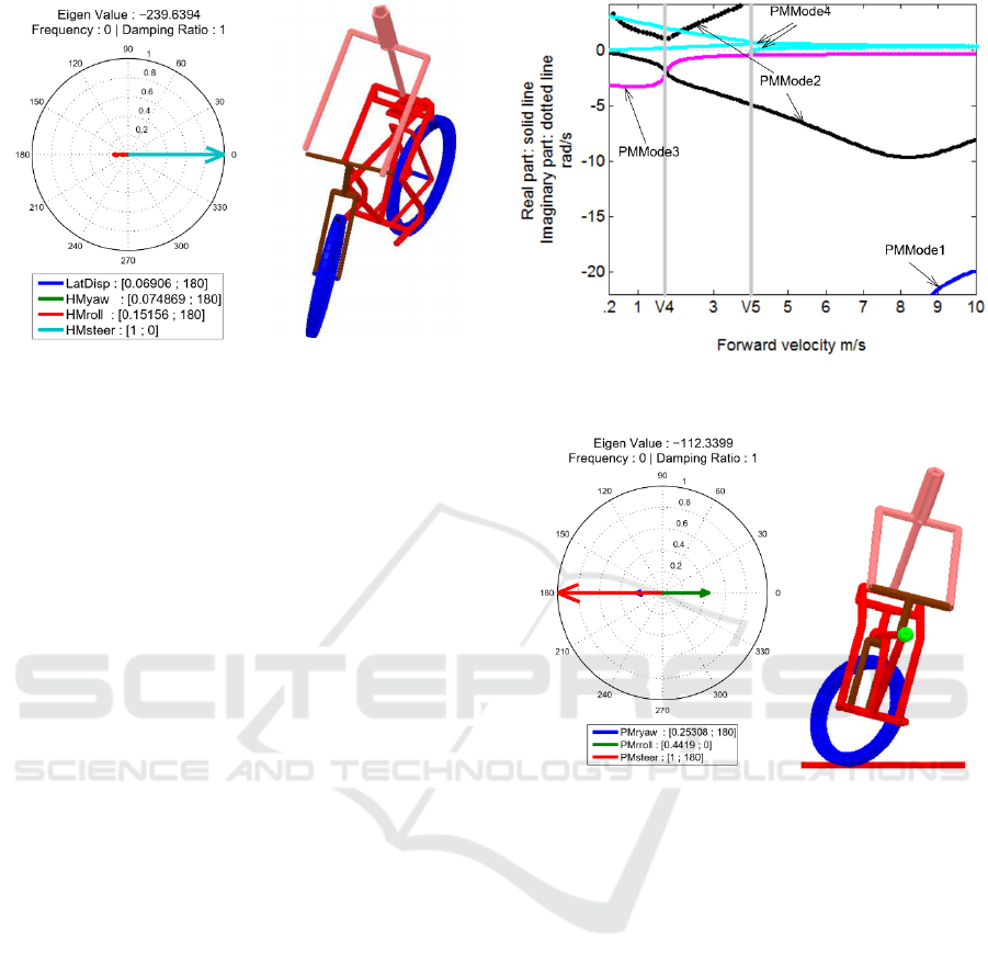
Figure 6: HMMode1 shape (right) and screenshot of its

vibrational motion (left) at 2 m/s.

This faster mode is responsible of the counter

steering phenomenon. In this investigated mechanical

model, HMMode1 is stable and non-oscillatory as the

wobble mode of a simplified motorcycle (Cossalter

and Roberto, 2015). The unstable and oscillatory

wobble encounter in bicycle model is due to the

implementation of the front frame flexibility and the

tire dynamics (Sharp, 2008; Dressel and Rahman,

2010).

Moreover, HMMode3 has an eigenvalue equal to

zero and characterized by a large lateral displacement

as HMMmode4. This behaviour is observed also with

HMMode4 and 5 when they are close the HMMode3

(below 4.2 m/s and above 5.5 m/s, respectively).

3.3 Modes of the Pedal Module Alone

The six eigenvalues computed exhibit four distinct

pedal module modes denoted from PMMode1 to 4.

Their evolutions over the forward speed are given in

Fig. 7.

Furthermore, PMMode1 to 3 are stable modes

whereas PMMode4 is the only unstable mode.

PMMode1 is also non-oscillatory like HMMode1

but slower with time constant value varying from 6E-

4 to 5E-2 second. It is characterized by a roll motion

in antiphase with those of the yaw and steer angles.

This can be seen on the mode shape in Fig. 8 (left).

Below 8.6 m/s, the steer motion is the dominant one;

and above this speed the roll motion become

dominant. This antiphase configuration feature

between the roll and the steer angles characterizes the

steer into the lean manoeuvre required to keep the

pedal module in equilibrium. Which means that the

rear steered handlebar play its designed role. The

steer into the lean manoeuvre is illustrated in Fig. 8

(right).

Figure 7: PM modes evolution over the forward the forward

speed range.

Figure 8: PMMode1 shape (right) and screenshot of its

vibrational motion (left) at 3 m/s.

In addition, PMMode2 behaves the same way as

PMMode1 but in an oscillatory manner with

frequencies varying from 0.64 Hz at the beginning of

the simulation process (at 0.2 m/s) to 3 Hz at 10 m/s.

A the forward speed of 1.7 m/s a frequency minimum

value of 0.17 Hz is reached together with a maximum

damping ration of 84%.

The yaw and the steer angle motions are the only

ones involved in PMMode3 and PMode4. PMMode3

is a non-oscillatory mode whereas PMMode4 is a

quasi-oscillatory one above V5 = 4.1 m/s. This

unstable begins with two non-oscillatory branches

that merge at V5 in an oscillatory form with a

maximum frequency equal to 5.7E-2 Hz reached at

8.8 m/s. The yaw and steer motions evolves in (quasi)

antiphase configuration for these pedal module

modes (see Fig. 9 (left)). The screenshot of

PMMode4 shown in Fig. 9 (right) suggests that as

time increases, higher yaw angle will be reached

(indeed slowly) due to the unstable nature of this

Numerical Investigation of the Lateral Dynamic Behaviour of the Anaconda

323

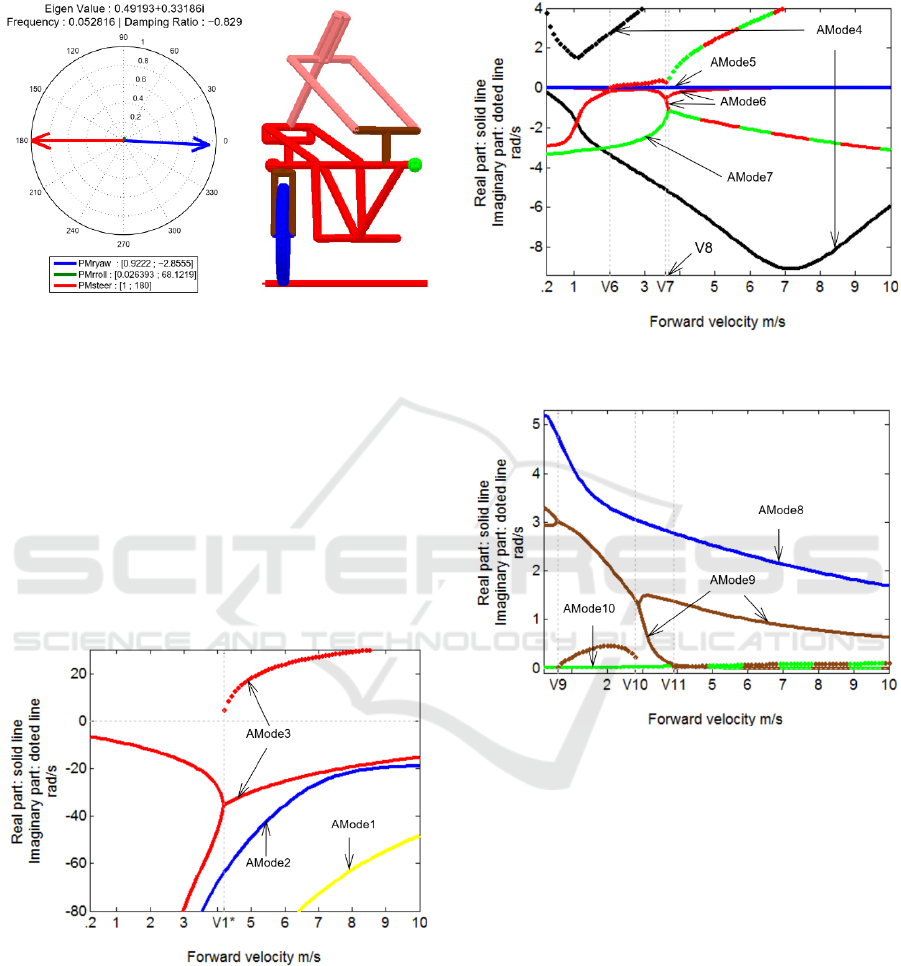
mode. This will lead the pedal module to hit the front

one.

Figure 9: PMMode1 shape (right) and screenshot of its

vibrational motion (left) at 3 m/s.

3.4 Modes of the Anaconda with One

Pedal Module

From the fourteen eigenvalues computed, only ten

distinct modes are found out to be distinct for the

Anaconda with one pedal module. They are denoted

from AMode1 to 10. Figs. 10, 11 and 12 depict the

evolutions of their eigenvalues with the forward

speed.

The first figure (Fig. 10) is concerned with stables

modes having lower time constant in the speed range.

Figure 10: First group of stable modes of the Anaconda

(AMode1, AMode2 and AMode3).

Moreover, each mode of the Anaconda with one

pedal module is found out to be a combination of one

mode of the head module and another one of the pedal

module; the head and the pedal modules being

considered alone as mentioned above.

Fig. 11 and 12 illustrate the remainder stable

modes and the unstable ones respectively.

Figure 11: Second group of stable modes of the Anaconda:

AMode4, AMode5, AMode6 and AMode7.

Figure 12: Unstable modes of the Anaconda: AMode8,

AMode9 and AMode10.

In summary, Tab. 3 relates each Anaconda mode with

its combination.

In addition, AMode1 and AMode2 are non-

oscillatory evolving over the speed range with an

increasing time constants like HMMode1 and

PMMode1.

AMode3 is oscillatory and a replication of

HMMode2. The weak influence of the pedal module

on this mode can be observed on shapes of both

modes (see Fig. 13). In these modes, the dominant

motion is the one of head module yaw angle.

AMode4, AMode5 and AMode10 are other cases of

complete replication of a mode over the speed range.

Particularly, Fig. 14 shows the replication of

PMMode2 in AMode4.

SIMULTECH 2021 - 11th International Conference on Simulation and Modeling Methodologies, Technologies and Applications

324

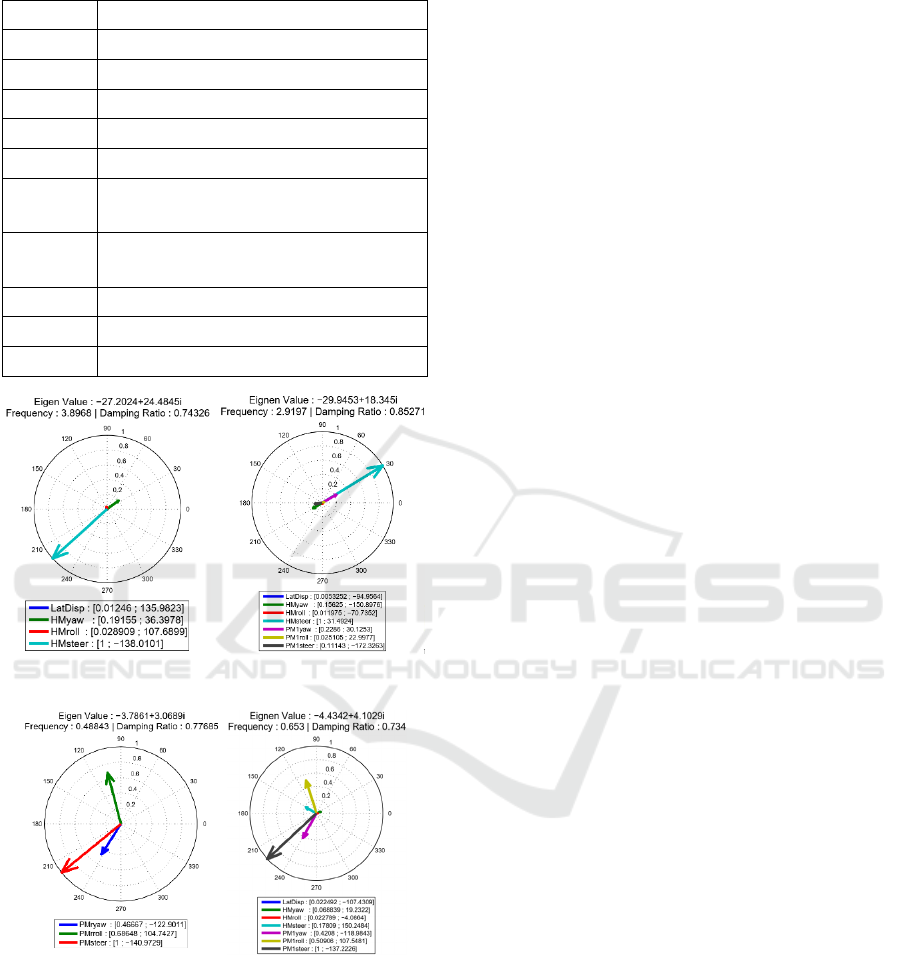
Table 3: Anaconda modes combinations.

AMode Combination

AMode1 HMMode1 + PMMode1

AMode2 HMMode2 lower branch + PMMode1

AMode3 HMMode2 + fixed pedal module

AMode4 fixed head module + PMMode2

AMode5 HMMode3 + fixed pedal module

AMode6 fixed head module + PMMode3 (v < V6)

Deformed shape of AMode6 (V6 < v < V7)

AMode7 HMMode5 + fixed pedal module (v < V7)

HMMode5 + PMMode3 (v > V7)

AMode8 HMMode5 + PMMode4

AMode9 HMMode6 + PMMode4

AMode10 fixed head module + PMMode4

Figure 13: Shapes of HMMode2 and AMode3.

Figure 14: Shapes of PMMode2 and AMode4.

Indeed, AMode6 begins with two non-oscillatory

branches below V6 = 2 m/s (replication of PMMode3

for the lower branches). These branches merge at this

speed in a quasi-oscillatory form up to V7 = 3.6 m/s.

In this speed range, the replication of PMMode3 is

slightly deformed by the presence of the lateral

displacement motion in anti-phase with the one of the

pedal module steer angle and in quasi-phase with the

one of the pedal module yaw angle. Beyond V8,

AMode7 is non-oscillatory and a replication of

HMMode5. From this speed, it merges with the lower

branch of AMode6 in an oscillatory form. In this

latter form, modes HMMode5 and PMMode3 are

combined.

It is emphasized that when the real part of an

eigenvalue is close to zero, the corresponding mode

shape is characterized by a dominant lateral

displacement motion.

The capsize (HMMode5) and weave HMMode6)

are the bicycle modes involved in the combination of

the unstable modes of the Anaconda: AMode8,

AMode9 and AMode10. Except AMode8 which

evolves over the speed range in a non-oscillatory

manner, AMMode9 and AMMode10 switch from one

form to another over the speed range (V9 = 0.6 m/s,

V10 = 2.9 m/s and V11 = 3.9 m/s).

They are known to be controllable at any forward

speed. Their combination with PMModes4 yields

unstable modes with real parts below 5 rad/s (but still

decreasing with the forward speed); so as the unstable

modes of the Anaconda can be controlled in the

human capabilities.

4 CONCLUSIONS

This study is concerned with the out-of-plane

dynamic of an Anaconda with one pedal module. The

linearization of nonlinear equations of motion of the

vehicle around a stationary state is required and

numerical simulations are carried out for some

forward speed in a speed range to get more insight in

the lateral behaviour of the Anaconda. All these tasks

are accomplished thanks to a co-simulation process

between EasyDyn and Matlab. Taking advantage of

the dynamic behaviours of the Anaconda’s

components it was found out that component modes

are combined each other or replicated in order to form

the one of the Anaconda. Particularly, the only one

unstable mode of the pedal module considered alone

is involved in the Anaconda’s unstable modes. The

analysis of the evolution of these unstable modes of

the Anaconda help to draw conclusions that tackle a

control issue for driving the Anaconda by human

drivers.

ACKNOWLEDGEMENTS

Authors are grateful to the School of Engineering’s

Department of the University of Quebec in Abitibi-

Témiscamingue.

Numerical Investigation of the Lateral Dynamic Behaviour of the Anaconda

325

REFERENCES

Verlinden, O., Kabeya, T. P., 2012. Presentation and

assessment of rideability of of a novel single track

vehicle: the Anaconda. Vehicle System Dynamics

(ISSN: 0042-3114), vol. 50, no. 8, pp. 1297-1317.

Kabeya, T. P., Verlinden, O., 2010. Simulation and Control

of the Anaconda. Proceeding of the Bicycle and

Motorcycle Dynamics, Symposium on the Dynamics

and Control of Single Track Vehicles, 20-22 October

2010, Delft, The Netherlands.

Sharp, R. S. (1971). The stability and control of

motorcycles. Proceedings of the IMechE, Part C,

Journal of Mechanical Engineering Science, 13:316–

329.

Limebeer, D. J. N., Sharp, R. S., 1971. Bicycles,

motorcycles and models: Single-track vehicle modeling

and control. IEEE Control Syst. Mag., 26(5):34–61.

Sharp, R. S., 1985. The lateral dynamics of motorcycles and

bicycles. Vehicle System Dynamics, 14:265–283.

Cossalter, V., 2006. Motorcycle Dynamics. Lulu, second

edition.

Meijaard, J. P., Papadopoulos, J. M., Ruina, A., and

Schwab, A. L., 2007. Linearised dynamics equations

for the balance and steer of a bicycle: a benchmark and

review. Proceeding of the Royal Society A:

Mathematical, Physical and Engineering Sciences,

463(2084):1955–1982.

Verlinden, O., Kouroussis, G., and Conti, C., 2005.

Easydyn: a framework based on free symbolic and

numerical tools for teaching multibody

systems. In Proceedings (on CD) of the ECCOMAS

Thematic Conference Multibody Dynamics, Madrid,

Spain.

Verlinden, O., Ben Fékih, L., and Kouroussis, G., 2013.

Symbolic generation of the kinematics of multibody

systems in EasyDyn: From MuPAD to Xcas/Giac.

Theoretical and Applied Mechanics Letters,

3(1):013012.

Kabeya, P., Verlinden, O., 2011. Application of

the multibody approach to the modeling of the

Anaconda. In Proceedings of the MULTIBODY

DYNAMICS, ECCOMAS Thematic Conference,

Brussels, Belgium.

MathWorks, T. I. 2005. Matlab version 7.1.

Koenen, C., 1983. The Dynamic Behaviour of a Motorcycle

when running straight ahead and when cornering. PhD

thesis, Delft University.

Kooijman, J., Schwab, A., Moore, J. K., 2009. Some

observations on human control of a bicycle. In

Proceedings of the ASME, International Design

Engineering Technical Conferences & Computers and

Information in Engineering Conference IDETC/CIE,

page 8 pp, San Diego, California, USA.

Cossalter, V., Roberto, L., 2015. Dynamics of motorcycle.

http://www.dinamoto.it/dinamoto/index_eng.html.

[Accessed online 2015-03-07].

Sharp, R. S., 2008. On the stability and control of the

bicycle. Applied Mechanics Reviews, 61(6):1–24.

Dressel, A. E., Rahman, A., 2010. Measuring dynamic

properties of bicycle tires. In Proceedings of Bicycle

and Motorbike Dynamics 2010, Symposium on the

Dynamics and Control of Single Track vehicles, Delft,

The Netherlands.

SIMULTECH 2021 - 11th International Conference on Simulation and Modeling Methodologies, Technologies and Applications

326