Empirical Evaluation of a Novel Lane Marking Type for Camera and

LiDAR Lane Detection

Sven Eckelmann

, Toralf Trautmann

, Xinyu Zhang

and Oliver Michler

Institute of Trafﬁc Telematics, Technical University Dresden, Dresden, Germany

Mechatronics Department, University of Applied Science Dresden, Dresden, Germany

Keywords:

LiDAR, Point Clouds, Retro Reﬂecting, Lane Marking, 3M, Camera.

Abstract:

Highly automated driving requires a zero-error interpretation of the current vehicle environment utilizing state

of the art environmental perception based on camera and Light Detection And Ranging (LiDAR) sensors. An

essential element of this perception is the detection of lane markings, e.g. for lane departure warnings. In this

work, we empirically evaluate a novel kind of lane marking, which enhances the contrast (artiﬁcial light-dark

boundary) for cameras and 3D retro reﬂective elements guarantee a better reﬂection for light beams from a

LiDAR. Thus intensity of point data from LiDAR is regarded directly as a feature for lane segmentation.

In addition, the 3D lane information from a 2D camera is estimated using the intrinsic and extrinsic camera

parameters and the lane width. In the frame of this paper, we present the comparison between the detection

based on camera and LiDAR as well as the comparison between conventional and the new lane marking in

order to improve the reliability of lane detection for different sensors. As a result, we are able to demonstrate

that the track can be detected safely with the LiDAR and the new lane marking.

1 INTRODUCTION

Highly automated driving requires a zero-error inter-

pretation of the current environment. Camera, radar,

ultrasound and LiDAR sensors are primarily utilized

for environmental perception and the detection of ob-

jects. In order to increase the reliability of said sen-

sors, competing and cooperative fusion approaches

can be applied. At the same time, the determina-

tion of the current position based on Global Naviga-

tion Satellite System (GNSS) sensors in combination

with vehicle data, such as velocity, rotational speed of

wheel and yaw rates is indispensable.

A precise information about the course of the lane is

an essential prerequisite for driver assistance systems

and autonomous driving and can further be used to

support global positioning. Besides the comfortable

lateral guidance, it serves as a reference point for fur-

ther driving maneuvers such as lane change assistance

or the calculation of alternative trajectories. Lane de-

tection based on camera information has already been

sufﬁciently handled and represents the current state of

the art. Next to these conventional image processing

algorithms, new approaches of machine learning are

adopted. However, the basis for these types of eval-

uation strategies is the 2D camera, so that the 3D in-

formation are estimated by the intrinsic and extrinsic

camera parameters as well as the known lane width.

This estimation is accompanied by numerous false de-

tection. Examples are glare, bitumen joints or other

elements that create a similar contrast in the image

(Koch et al., 2015).

1.1 Related Works

1.1.1 LiDAR Lane Detection

In literature, several approaches have been proposed

using LiDAR as an input for lane detection. In

(Kammel and Pitzer, 2008) the disadvantage of low

resolution is compensated by increased subsequent

scans, registered and accumulated employing GNSS

and Inertial Measurement Unit (IMU) information.

The authors in (Hata and Wolf, 2014) used a modi-

ﬁed Otsu thresholding method and were able to detect

lanes and any kind of road painting. In (Kodagoda

et al., 2006) a sensor fusion algorithm to fuse images

from camera and scanning laser radar (LADAR) is

used to identify curbs. For this task, the solution pre-

sented in this paper used nonlinear Markov switch-

ing. The authors in (Kumar et al., 2013) extracted the

lane lines by developing an algorithm that combines

Eckelmann, S., Trautmann, T., Zhang, X. and Michler, O.

Empirical Evaluation of a Novel Lane Marking Type for Camera and LiDAR Lane Detection.

DOI: 10.5220/0010550500690077

In Proceedings of the 18th International Conference on Informatics in Control, Automation and Robotics (ICINCO 2021), pages 69-77

ISBN: 978-989-758-522-7

both Gradient Vector Flow (GVF) and Balloon Para-

metric Active Contour models. This technique was

not very accurate to detect lanes at the edges of the

road and the lane predicted interfered with the road

curbs. The same author published a lane detection

algorithm (Kumar et al., 2014) based on an inten-

sity threshold as well as Region Of Interest (ROI) to

limit the number of processed LiDAR data. Subse-

quently, the data was converted to a 2D image, with

a linear dilation to complete rubbed off lanes. The

algorithm was tested over 93 roads and managed to

detect the markings in 80 roads. The authors claimed

that the failures in detecting all the test roads was due

to road wipings and erosion, causing small intensi-

ties and low densities to be received by the LiDAR.

In (Guan et al., 2014) the point cloud is segmented

into horizontal blocks. These blocks are then used

to detect the edges (road curbs) based on differences

in elevation in order to determine the surface as well

as the road boundaries. The authors claim to accom-

plish a success of 0.83 of correctness to detect lane

markings. In (Thuy and Le

on, 2010) the authors de-

veloped a lane marking detection algorithm based on

a dynamic threshold. First, the data points received

from the LiDAR is processed using Probability Den-

sity Function (pdf), and the maximum reﬂectively is

matched with the highest values of the pdf. The dy-

namic threshold is applied to this reﬂectively data,

since the lane markings are the ones that return high

reﬂectively (due to their color gradient). The author

of (Yan et al., 2016) transformed the segmented points

into scan lines based on scanner angle. Consequently,

the road data is determined based on a ”Height Dif-

ference” (HD). The road limits have been identiﬁed

with a moving least square, that only accepts certain

points that lie in a certain threshold set by the authors.

Besides a classiﬁcation on intensity values, the au-

thors proposed using an ”Edge Detection and Edge

Constraints” (EDEC) technique that detects ﬂuctua-

tions in the intensity. This method should minimize

the noise in the detected lanes. The algorithm was

tested on data from Jincheng highway China, the au-

thors claim that they have accomplished an accuracy

level of 0.9.

1.1.2 Camera Lane Detection

Camera based lane marking detection research is a

main research ﬁeld and currently heavily studied.

Therefore in this section, only a brief overview of re-

lated works is provided. The lane detection algorithm

in (Mu and Ma, 2014) converts the raw images to grey

scale and applies a Otsu’s method for thresholding the

image. Sobel is used to detect the lane markings. The

results shows that it is effective for incomplete lane

markings and for ﬂuctuations in the environment’s il-

lumination. (Li et al., 2014) uses Canny edge detec-

tion technique which results in a binary image. Then

Hough transform is implemented in order to detect the

straight lines from the image. In contrast, the author

of (Haque et al., 2019) uses thresholding based on

gradients and the HLS color space. Followed by the

perspective transformation they apply a sliding win-

dow algorithms. The centroids of the windows a ﬁ-

nally composed to a lane.

1.2 Our Approach

For the approach presented in this paper, we tackle

the main problem where lane detection in urban areas

often fails, since the curving of the lane runs out of

the scope from the camera. In addition most of the

algorithms are mostly designed for straight lanes and

not for sharp curves. Thus a reliable lane information,

one of the basics for autonomous driving, is not guar-

anteed. In this paper we use a new type of lane mark-

ing which was developed by 3M (3M, 2021). This

lane marking enhances the contrast (artiﬁcial light-

dark boundary) for camera systems and the reﬂecting

of light beam from a LiDAR with 3D arranged retro

reﬂective elements. The intensities of the point data

can directly be used as a feature for the segmenta-

tion. Complex ﬁlters are not required to extract the

information from the lane marking and misinterpre-

tations are minimized. With transferring the LiDAR

points into the 2D area, the lanes are then extracted

through dynamic horizontal and vertical sliding win-

dows, which ﬁnally leads to the relevant points. For a

better comparison we take the raw points into account

and will not apply any ﬁlters for a smooth represen-

tation. It will also provide a comparison between the

detection based on camera and LiDAR. All the mea-

surements are done on the test ﬁeld of the University

of Applied Science (HTW) Dresden. Since only one

lane is equipped with this new lane marker, a compar-

ison to the conventional lane marking can be given.

2 FUNDAMENTALS

2.1 LiDAR

A LiDAR emits infrared coherent light from a laser to

its environment. The energy is decisive for the clas-

siﬁcation of the sensor into the protective classes and

results from the integral of the pulse over time. Due to

the optics of the LiDAR, the light beam diverges and

spreads ﬂat, depending on the distance. This means

that less light power is radiated onto the object in a

ICINCO 2021 - 18th International Conference on Informatics in Control, Automation and Robotics

further distance. In addition particles in the atmo-

sphere, like dust, fog and rain cause diffuse reﬂec-

tions and absorb energy from the ray. Furthermore,

the surface of the object inﬂuences the reﬂected en-

ergy. Physical properties like total and diffuse reﬂec-

tion along with the kind of color have a signiﬁcant

impingement. In contrast to the source of the LiDAR,

the light beam is reﬂected from the object with a full

solid angle and is signiﬁcantly attenuated by the scat-

tering of infrared light. After all, the sensitivity and

surface size of the receiver inﬂuence the result of the

detection (Wagner et al., 2003).

The transmittance of the LiDAR is the quotient be-

tween the transmitted and the received light output.

This value is colloquially known as intensity. In or-

der to minimize the inﬂuence of attenuation by the

atmosphere, the transmission power can be increased

or the beam can be bundled more stronger. Another

approach is to change the composition of the object

color. Therefore BASF Coatings announced a new

technology called cool colors or cool coatings (Coat-

ings, 2016). This technology replaces a high propor-

tion of ash in the paint and can reﬂect energy better. In

addition to the cooler interior in the vehicle, LiDAR

beams are also better reﬂected. The distance d to an

object is calculated by the speed of light c and half of

the appertaining run time t:

d = c

·t/2 (1)

In summery, the LiDAR is the sensor with the high-

est accuracy, but with increasing distance and the re-

sulting minimization of the object-relevant back scat-

ter pulse, the reliability and integrity of object detec-

tion reduces. At the same time, object properties such

as surface texture, deﬁned in color and gloss, relative

orientation and atmospheric properties affect the back

scatter intensity of the LiDAR.

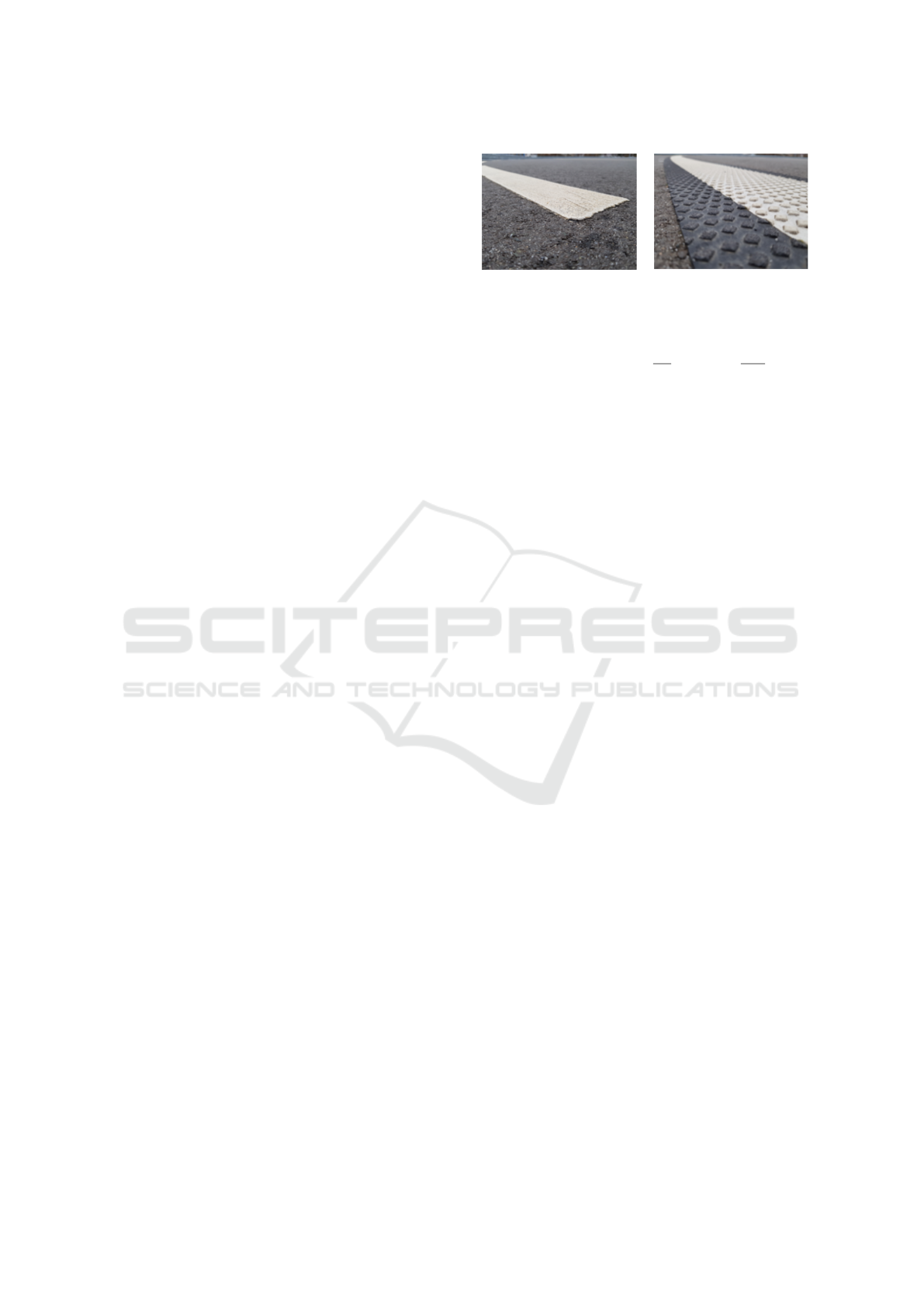
2.2 Lane Markings

The examined novel type of lane marker tapes (3M,

2021) (Figure 1) have retro reﬂective characteristics,

which are achieved by embedding glass beads. Inci-

dent light in this direction is scattered directly back.

The black stripe increases the contrast to the white

lane marking and therefore provides a deﬁned con-

trast. This is particularly helpful on light surfaces,

such as concrete. With the tall design, better visibil-

ity in rain and snow should be achieved. Originally,

they were developed to improve recognition by hu-

man drivers or a camera.

The visibility in daylight as well as the retro re-

ﬂective properties are deﬁned by the Luminance Co-

efﬁcient Q

or R

2, which is the quotient of Lumi-

ance Density L

[

] and Illumiance E

[lx].

Figure 1: Left: Standard Lane Marking Right: Retro reﬂec-

tive lane marking tape of 3M (3M, 2021) with embedded

glass beads.

[

mcd

] (2)

is deﬁned in EN 1436, 2007 which deﬁnes mini-

mum Luminance Coefﬁcents in different classes de-

pending on the color of the road marking, the kind

of surface (alphalt or concrete) and the dampness. In

addition to the new markings on the outer lane, the

conventional markings are applied to the center lane

and the inner lane on the test ﬁeld. The retro reﬂective

marking has a seven times higher Luminance Coefﬁ-

cient of R

= 352 comparing to the conventional

lane marking of R

conv

= 50.

3 EXPERIMENTAL SETUP

3.1 Vehicle

For the investigations a BMW i3 is used as test vehi-

cle. Additional information like vehicle speed, steer-

ing angle and wheel speed are directly provided from

the car via a CAN interface. All information are cap-

tured by a mini PC over Ethernet and uniquely time

stamped. Thus it is possible to play back the data at a

later time and to optimize the implemented algorithm.

3.2 LiDAR

For the approach, the LiDAR system Ouster OS1 is

used. With a range of 120 m, a 360

◦

horizontal ﬁeld

of view and a given angular resolution of 0.1

◦

as well

as a

/- 22.5

◦

vertical ﬁeld of view divided into 64

levels, it generates up to 1.310.720 points per second

with a sampling frequency of 20Hz (Ouster, 2014).

The LiDAR is mounted at a height of 1.8 m. Figure 2

shows the point data from the LiDAR of a measure-

ment.

The LiDAR as well as a GNSS receiver is

mounted on a mobile platform, which can easily be

adapted to the roof of different vehicles.

Empirical Evaluation of a Novel Lane Marking Type for Camera and LiDAR Lane Detection

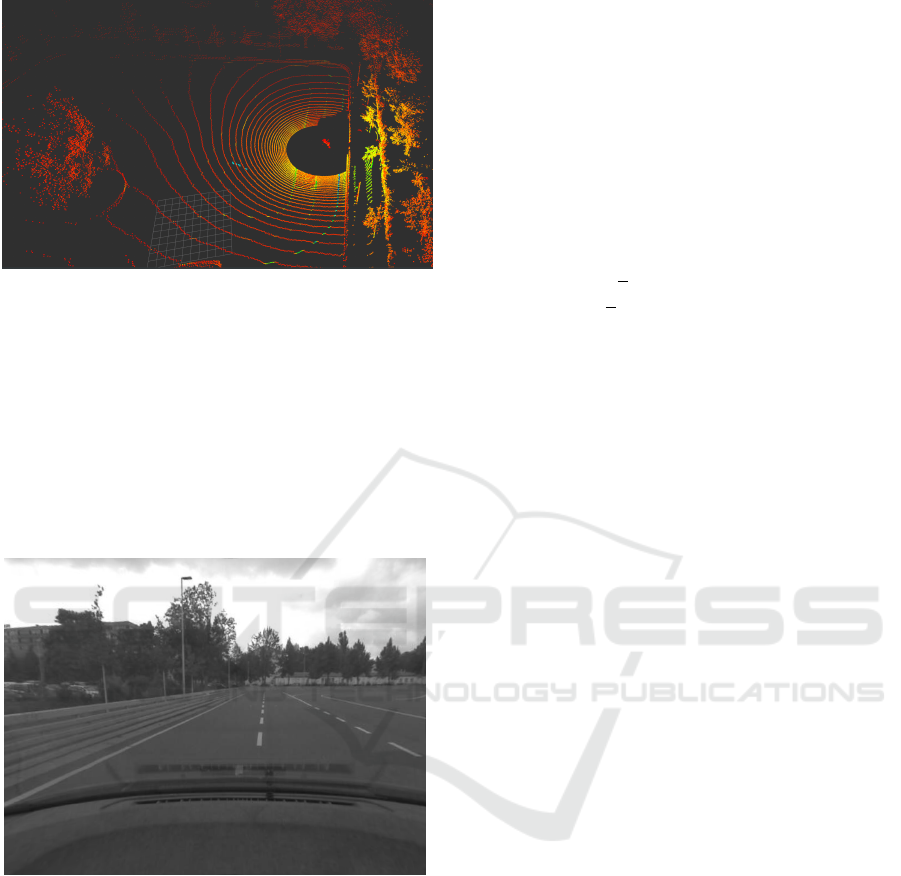
Figure 2: Recorded point cloud of a straight street on the

reference track with a LiDAR sensor. The outer line is

equipped with the retro reﬂecting lane from 3M.

3.3 Camera

In addition, a camera-based lane marking detection is

evaluated. The camera used in this work is a grey

scale camera (Axis M3114-R) with a resolution of

640x480 pixels. It is mounted in the center of wind-

shield, close to the roof. A sample of the camera’s

raw image is shown in ﬁgure 3.

Figure 3: Rectiﬁed gray scale image frame of AXIS

M3114-R (640x480).

3.4 Reference Positioning System

In order to provide a geo-reference as well as a quan-

titative comparison between the examined lane de-

tection methods, the current position of the vehicle

must be determined as precisely as possible. For this,

an u-blox multi-constellation GNSS receiver (ublox,

2017) is utilized to estimate the current global po-

sition. They include already integrated fusion algo-

rithm to countervail the current GNSS error. In our

case we use the automotive and static setting to en-

courage a low deviation and thus a reliable position.

In addition we combine the output from the GNSS

modules with information provided by the vehicle

CAN bus system, which are the current vehicular ve-

locity v and the yaw rate ψ. The absolute position x,y

and the heading of the vehicle Θ are calculated by an

Extended Kalman Filter (EKF). The state vector x

ctrv

of the fusion model is described in 3. For the applied

prediction motion model we use a Constant Turn Rate

and Velocity (CTRV) model (equation 4) described in

(Obst et al., 2015).

ctrv

= (x,y, Θ,v,ψ) (3)

k+1

= x







∗ (sin(Θ + ψ ∗ T ) − sin(Θ))

∗ (−cos(Θ + ψ ∗ T ) + cos(Θ))

Θ ∗ ψ ∗ T







(4)

3.5 Test Field with Reference Track

The equipped and examined track (ﬁgure 4) is part of

the test ﬁeld from the University of Applied Science

located in Dresden, Germany. It has a dimension of

approximately 50 m by 70 m. Contrary to common

available data, like Open Street Map (OSM), the test

ﬁeld is geodetically surveyed with an high accuracy.

In addition we are able to map lanes, intersections and

we are able to set geographical referenced markers.

The red coordinate system depicted in ﬁgure 4 repre-

sents the origin point of the local map. The surveyed

data acquisition includes a complete lap around the

outer test track. In addition to the LiDAR data, the

data set also contains the relative position in relation

to our coordinate origin (red) and raw camera data.

4 DATA PROCESSING

4.1 Camera Lane Detection

The whole workﬂow is given in ﬁgure 5. After recti-

fying the raw image in the ﬁrst step, we set the ROI

from the lower edge of the windshield up to the hori-

zon, which is approximately the half of the image. In

this ROI we improved the contrast and minimized the

inﬂuence of ambient lighting by taking the histogram

of this region in account.

A Canny edge detector followed by an morpho-

logical operation for closing unﬁlled regions converts

the gray image to a binary. Finally we crop the im-

age again by setting vertices of a trapezoid to reduce

the inﬂuence of obstacles in the edge area. Up next,

ICINCO 2021 - 18th International Conference on Informatics in Control, Automation and Robotics

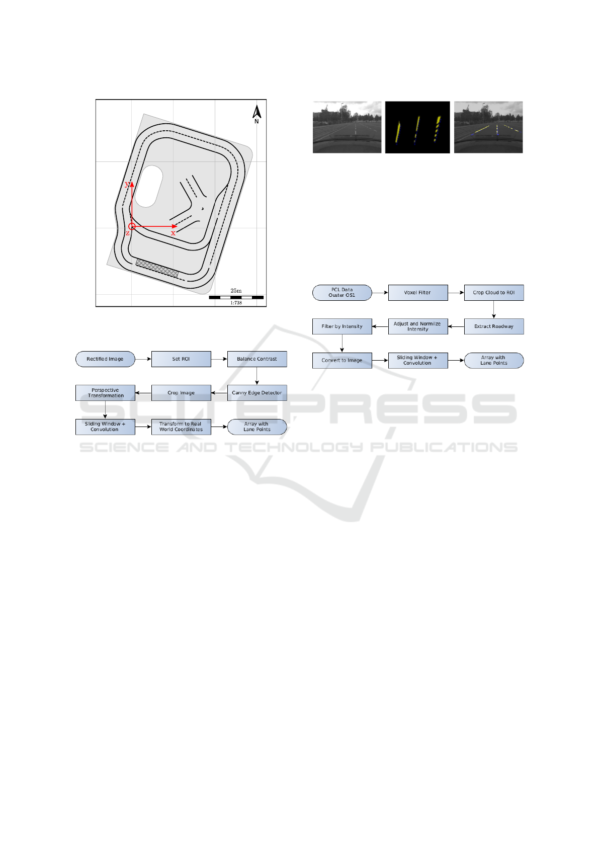
Figure 4: Reference track on the test ﬁeld. The red frame

represents the local coordinate system. The retro reﬂecting

lane marking is only applied to the outer lane.

Figure 5: Workﬂow of the camera lane detection.

we perform a perspective transformation, which re-

sults in a bird eye view image (ﬁgure 6, Center). This

image is the starting point for the lane detection algo-

rithm. Therefore, we are using a sliding window start-

ing from the lower left corner and moving horizontal

to the end of the image. In each window we are us-

ing convolution to detect the maximum of white pix-

els. By passing a threshold, the position of the max-

imum convolution becomes a valid point of the lane,

which we name centroid. Once we ﬁnd a centroid we

start going vertical in the image. Simultaneously we

use the orientation of the centroid to deﬁne the next

vertical window position. This vertical iteration ends,

once we ﬁnd no valid point and then start over from

the last horizontal position. The algorithm ends once

we reached the right side of the image. As result we

get the relevant points of the lanes in the bird’s eye

perspective. Finally we can augment our centroids

into the rectiﬁed image (ﬁgure 6, Right).

Figure 6: Examples of the camera lane detection. Left:

Original rectiﬁed image. Center: Binary image in bird eye’s

view. The yellow points represents the segmented points

and the blue points (centroids) are extracted by the sliding

window algorithm. Right: The segmentation (yellow) and

the centroids (blue) are augmented in the rectiﬁed image.

4.2 LiDAR Lane Detection

The entire workﬂow for LiDAR lane detection is

given in Figure 7.

Figure 7: Workﬂow of the LiDAR lane detection.

We process the raw point cloud data from the

LiDAR and start down sampling with a Voxel Fil-

ter and a leaf size of 0.2. We crop the point cloud

to predeﬁned ROI and focus on the relevant area in

front of the vehicle. A Random Sample Consensus

(RANSAC) is used to extract the roadway (cf. ﬁg-

ure 8, left image). Since the intensity value decreases

over the distance, we normalize and adjust that value

with a linear function. Finally we set a threshold, ex-

tract the remaining lane points and convert these to an

image. At this point we can use the same approach to

extract the lanes with a sliding window as described

in section 4.1. Finally we convert the lane points back

from the image plane to the vehicle coordinate sys-

tem and create optional a second degree polynomial

(cf. ﬁgure 8, right image).

5 RESULTS

Out of the approximated lane points and our current

known position (cf. section 3.4), we can transform

each point of our detection algorithm into the global

coordinate system, which is exemplary depicted in

ﬁgure 9.

Since our test ﬁeld and all lanes are geodetically

surveyed we are able to compare the results with the

ground truth. For evaluation and comparison, the

Empirical Evaluation of a Novel Lane Marking Type for Camera and LiDAR Lane Detection

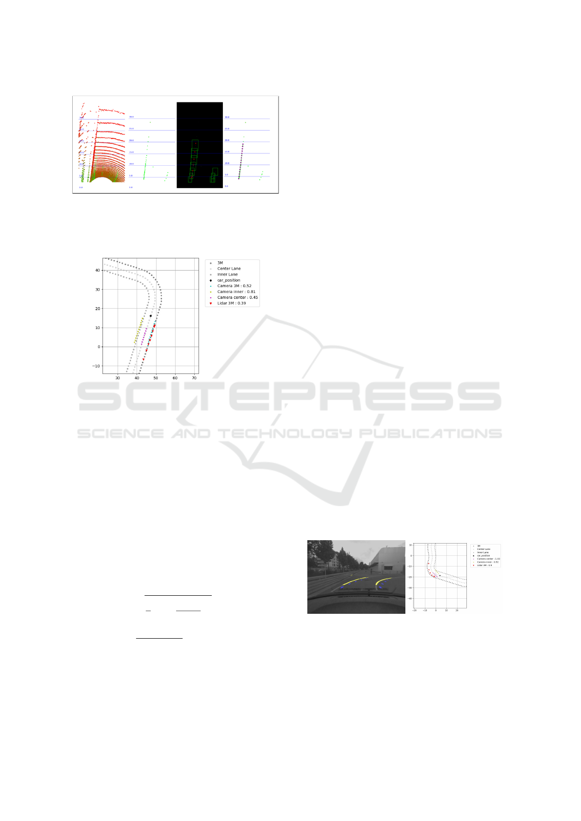
Figure 8: Examples for LiDAR Lane Detection. Form Left

to Right: Extracted roadway as top view image; Segmented

Lane with adjusted Intensity threshold; Extracting relevant

lane points with sliding window algorithm; Fitted points

(purple) with second degree polynomial.

Figure 9: Transformed lanes into the global coordinate sys-

tem. The ground truth is represented by the 3M -, Center-

and Inner Lane and the black cross marks the current car

position. The colored points represent the centroids of the

detected lanes. The values of the Camera and Lidar detected

lanes specify the Root Mean Square Error (RMSE) from the

ground truth.

maximum length of the lane l

Lane

, the deviation from

the ground truth RMSE and the fail rate f

(cf. equa-

tion 5) are assessed. The length l

Lane

is deﬁned as

the distance from the center point of the car up to

the farthest detected point. For calculating f

we de-

ﬁne that all lanes which have an higher deviation than

RMSE

max

count as not detected n

alse. Since we

have the same sample rate of our LiDAR and camera,

we also count the number of frames where no lane

was detected n

not

. Based on the evaluation of the test

drive, RMSE

max

is set to 1.5 m.

RMSE

Lane

i=1



− f



(5)

not

+ n

f alse

f rames

(6)

f alse

∑

Frames

n=0

(RMSE

Lane

> RMSE

max

)

(7)

5.1 Camera Lane Detection

The 3M marking can be used to examine if the con-

trast strip allows a better detection compared to con-

ventional lane markings. Figure 11 shows the devia-

tion from the ground truth for each lane and allows us

to make the following statements:

• Camera Fails in Curves: Especially in narrow

curves the lanes are running out of the cameras

ﬁeld of view. A detection of an inner lane mark-

ing is very unlikely. Only center and outer lane

markings could be detected. Due to the structure

of our text ﬁeld, there is a crash barrier near the

outer lane, which leads additionally to an incor-

rect detection.

• Incorrectly Assigned Lanes: The assignment of

each lane to the ground truth is done by calculat-

ing the RMSE of each point to the ground truth.

In that case, the course of the lane approaches the

other reference track (cf. ﬁgure 10). As a result,

the lanes were assigned incorrectly (cf. ﬁgure 11

at A).

• Low Deviation on Straight Lanes: In regions of

straight lanes the RMSE is lower than 1.0m.

• Uncertainty Due to Position Determination: In

B of ﬁgure 11 the car did not move along the cen-

ter line. Additionally the uncertainty of the posi-

tion determination caused a higher RMSE and a

false detection.

The error rate of the 3M marking is between the mid-

dle and inner lane. At this point we cannot assess

whether the 3M marking improves the lane detection,

since the inner lane runs out of the ﬁeld of view while

passing curves and the crash barriers often causes a

false detection. Furthermore, the roadway on the test

ﬁeld is already very dark, so that only a minimal im-

provement in the contrast can be achieved.

Figure 10: Error due transforming the points from the cam-

era coordinate system into the global coordinate system.

5.2 LiDAR Lane Detection

As already mentioned, the LiDAR lane detection only

takes the retro reﬂecting lane markings into account.

ICINCO 2021 - 18th International Conference on Informatics in Control, Automation and Robotics

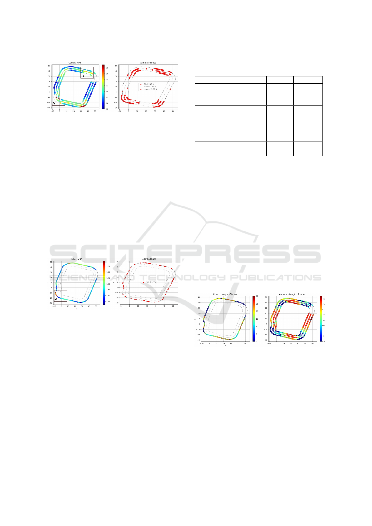
Figure 11: Left: RMSE from each lane to the ground truth.

None colored regions are areas there the algorithm didn’t

detect any valid lane points n

f alse

.Right: Represents the fail

rate of the camera detection on each lane.

Thus, only the outer lane can be evaluated. Based on

ﬁgure (12) we can point out the following statements:

• Low Fail Rate: The false detection is equally dis-

tributed on the whole track. In region A of ﬁg-

ure 12 the detection fails because the segmenta-

tion returns a high intensity due to retro reﬂecting

objects. The overall fail rate is f

Lidar

= 7.94%

• Correctly Assigned Lanes: The extracted lane

points were assigned to the outer lane in each

frame.

• Low Deviation: The deviation along the whole

track is below 1 m. It only raises at regions where

the segmentation process failed due of high inten-

sity obstacles.

Figure 12: Lidar Lane Detection - Left: RMSE of the 3M

lane to the ground truth. None colored regions are areas

where the algorithm was not able to detect any valid lane

points n

f alse

. Right: Fail rate of the LiDAR lane detection

on each lane.

5.3 Comparison of LiDAR and Camera

Figure 13 shows the length of the detected lanes. The

maximum of the LiDAR and thus the prediction hori-

zon is l

Lane

Lidar

= 30m, compared to the camera with

Lane

Camera

= 16m. The lower installation position of

the camera, creates a higher perspective distortion.

Therefore, the area of the image, which represents the

roadway and the lanes is smaller. That leads to the

fact, that only few points in a smaller area can be used

for subsequent processing. In addition the transfor-

mation from birds-eye-view to real coordinates fails

in narrow curves, which leads to a wrong assignment

of the lane (ﬁgure 10). Currently, only the camera is

Table 1: Final results of the comparison between the LiDAR

and camera lane detection.

LiDAR Camera

Max Length of Lane [m] 31 16

Fail Rate of Conventional

Lane Marking [%]

– 22,26

Fail Rate of 3M Lane

Marking [%]

7.9 22,68

Average RMSE of

Conventional

Lane Marking [m]

– 0.86

Average RMSE of 3M

Lane Marking [m]

0.76 0.88

able to detect multiple lanes. If we deﬁne the error

rate in such a way, that at least one marking has to

be recognized, the fail rate drops to 1%. The LiDAR

is mounted on the roof of the car and already pro-

vides 3D data. So any perspective transformation

steps do not need to be performed. The resolution of

the LiDAR based on the design of the LiDAR system.

In relation to our LiDAR, the vertical ﬁeld of view is

divided into 64 layers. The blind areas between the

layers increases with the distance. As result, fewer

points in the lane are recorded and changes in between

can not be perceived. That also leads to the fact the

the maximum length, and thus the prediction horizon

depends on the visibility of each speciﬁc layer. Com-

pared to this, the camera has a ﬁxed and usually a

higher resolution. In subject to the condition that the

whole marking is visible, changes in the course of the

trajectory can be better recognized.

Figure 13: Length of Lane Detection - Left: Lidar Right:

Camera.

Concluding, table 1 provides a comprehensive

overview of all quantitative results.

6 CONCLUSION AND FUTURE

WORKS

In this paper we compared a new type of lane mark-

ing (3M, 2021) using a LiDAR(Ouster OS1 (Ouster,

2014)) sensor with a camera-based lane detection.

With varieties in data processing steps and coordinate

Empirical Evaluation of a Novel Lane Marking Type for Camera and LiDAR Lane Detection

transformations, the same lane detection algorithm is

applied for both sensors. The paper shows that the

new lane marking together with the LiDAR gives the

best results. The length of the predicted lane is two

times higher and the fail rate is less than one third

of the camera. It also shows, due the cameras lim-

ited ﬁeld of view, narrow curves can not be detected

as well. The new lane marking did not improve the

detection algorithm of the camera at all. This is ba-

sically due to the already dark pavement of the test

ﬁeld. For future work, we will invest more research

in the following topics.

• Various Undergrounds: Evaluating the inﬂu-

ence of the contrast stripe on brighter roadways

like concrete.

• Various Weather Condition: Since the new lane

marking has certain height, questions like how

rain and snow inﬂuences the detection should be

evaluated.

• Night Vision: It needs to be evaluated if the retro

reﬂecting inﬂuences the night visibility for the

camera detection.

• Combine with V2X Technology: A Road Side

Unit (RSU) could provide the information, if a

lane is equipped with this special feature. Under

the condition a vehicle is equipped with a LiDAR,

the detection of the lane could be supported and

serve as a prerequisite for highly automated driv-

ing.

• Sensor Fusion: A sensor fusion of camera and

LiDAR would increase the reliability of the lane

detection

Since 2020 where is new version of the 3M lane

marking on the market. We are looking forward to

equipped also the inner lane, which enables us to

compare the three variants.

Besides lane marking, pole feature has seen a

tremendous interest amongst research community in

recent years because of their ubiquity on the urban

street and stability under different weather and light

conditions. It appears normally as part of street light,

trafﬁc lights and trees. In a future work we will

present a new pole detection method, combining high

retro reﬂective foils and LiDAR, which enables the

calculation of lateral and longitudinal relative posi-

tion of the vehicle. The test ﬁeld is already equipped

with nine trafﬁc lights, which provides an excellent

basis for this investigation.

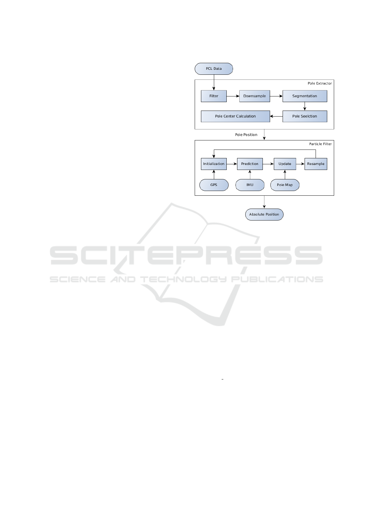
Figure 14 shows the ﬂow chart for the localization

process based on pole feature. It is divided in a Pole

Extractor and Particle Filter. After ﬁltering, down

sampling and segmentation, the point cloud data is

Figure 14: Flow chart for relative pose estimation with

LiDAR and poles.

extracted into multiple independent clusters. A pre-

deﬁned condition selects the relevant pole cluster and

with the transformation it into a 2D plane, it serves as

input for the localization process. Therefore we are

using a particle ﬁlter. The initial position and ground

truth are provided from GNSS sensor. The prediction

step uses the speed and yaw rate information which

are gathered from IMU. With the combination a the

lane detection algorithm and the pole extraction al-

gorithm we combine two position determination ap-

proaches, with the goal to enhance the autonomous

driving.

REFERENCES

3M (2021). 3m

stamark

high performance

contrast tape 380aw-5. https://www.3m.com/

3M/en US/company-us/all-3m-products/

∼

/3M-

Stamark-High-Performance-Contrast-Tape-380AW-

5/?N=5002385+8709322+3294235158&rt=rud.

Accessed: 20121-02-24.

Coatings, B. (2016). Basf cool coatings. https:

//www.basf.com/global/de/who-we-are/organization/

locations/europe/german-sites/Muenster/News-

Releases/BASF-erhaelt-Bundespreis-Ecodesign-

fuer-Cool-Coatings.html. Accessed: 2021-02-24.

Guan, H., Li, J., Yu, Y., Wang, C., Chapman, M., and Yang,

B. (2014). Using mobile laser scanning data for auto-

ICINCO 2021 - 18th International Conference on Informatics in Control, Automation and Robotics

mated extraction of road markings. ISPRS Journal of

Photogrammetry and Remote Sensing, 87:93–107.

Haque, R., Islam, M., Alam, K. S., Iqbal, H., and Shaik,

E. (2019). A computer vision based lane detection

approach. International Journal of Image, Graphics

& Signal Processing, 11(3).

Hata, A. and Wolf, D. (2014). Road marking detection us-

ing lidar reﬂective intensity data and its application to

vehicle localization. In 17th International IEEE Con-

ference on Intelligent Transportation Systems (ITSC),

pages 584–589. IEEE.

Kammel, S. and Pitzer, B. (2008). Lidar-based lane marker

detection and mapping. In 2008 IEEE Intelligent Ve-

hicles Symposium, pages 1137–1142. IEEE.

Koch, C., Georgieva, K., Kasireddy, V., Akinci, B., and

Fieguth, P. (2015). A review on computer vision based

defect detection and condition assessment of concrete

and asphalt civil infrastructure. Advanced Engineer-

ing Informatics, 29(2):196–210.

Kodagoda, K., Wijesoma, W. S., and Balasuriya, A. P.

(2006). Cute: Curb tracking and estimation.

IEEE Transactions on Control Systems Technology,

14(5):951–957.

Kumar, P., McElhinney, C. P., Lewis, P., and McCarthy, T.

(2013). An automated algorithm for extracting road

edges from terrestrial mobile lidar data. ISPRS Jour-

nal of Photogrammetry and Remote Sensing, 85:44–

55.

Kumar, P., McElhinney, C. P., Lewis, P., and McCarthy,

T. (2014). Automated road markings extraction from

mobile laser scanning data. International Journal

of Applied Earth Observation and Geoinformation,

32:125–137.

Li, Y., Iqbal, A., and Gans, N. R. (2014). Multiple lane

boundary detection using a combination of low-level

image features. pages 1682–1687.

Mu, C. and Ma, X. (2014). Lane detection based on object

segmentation and piecewise ﬁtting. TELKOMNIKA

Indones. J. Electr. Eng. TELKOMNIKA, 12(5):3491–

3500.

Obst, M., Hobert, L., and Reisdorf, P. (2015). Multi-sensor

data fusion for checking plausibility of V2V com-

munications by vision-based multiple-object tracking.

IEEE Vehicular Networking Conference, VNC, 2015-

Janua(January):143–150.

Ouster (2014). Ouster os1 datasheet. https://data.ouster.

io/downloads/OS1-lidar-sensor-datasheet.pdf. Ac-

cessed: 2021-02-24.

Thuy, M. and Le

on, F. (2010). Lane detection and track-

ing based on lidar data. Metrology and Measurement

Systems, 17(3):311–321.

ublox (2017). NEO-M8P u-blox M8 High Precision GNSS

Modules Data Sheet. Document Number UBX-

15016656, Revision R05, January 2017.

Wagner, W., Ullrich, A., and Briese, C. (2003). Der laser-

strahl und seine interaktion mit der erdoberﬂ

ache.

Osterreichische Zeitschrift f

ur Vermessung & Geoin-

formation, VGI, 4(2003):223–235.

Yan, L., Liu, H., Tan, J., Li, Z., Xie, H., and Chen, C.

(2016). Scan line based road marking extraction from

mobile lidar point clouds. Sensors, 16(6):903.

Empirical Evaluation of a Novel Lane Marking Type for Camera and LiDAR Lane Detection