Stability Analysis for State Feedback Control Systems Established as

Neural Networks with Input Constraints

Lukas Markolf

and Olaf Stursberg

Control and System Theory, Dept. of Electrical Engineering and Computer Science, University of Kassel,

Wilhelmsh

oher Allee 73, 34121 Kassel, Germany

Keywords:

Constrained Control, Intelligent Control, Neural Networks, Reinforcement Learning, Stability.

Abstract:

Considerable progress in deep learning has also lead to an increasing interest in using deep neural networks

(DNN) for state feedback in closed-loop control systems. In contrast to other purposes of DNN, it is in-

sufﬁcient to consider them only as black box models in control, in particular, when used for safety-critical

applications. This paper provides an approach allowing to use the well-established indirect method of Lya-

punov for time-invariant continuous time nonlinear systems with neural networks as state feedback controllers

in the loop. A key element hereto is the derivation of a closed-form expression for the partial derivative of

the neural network controller with respect to its input. By using activation functions of the type of sigmoid

functions in the output layer, the consideration of box-constrained inputs is further ensured. The proposed

approach does not only allow to verify the asymptotic stability, but also to ﬁnd Lyapunov functions which can

be used to search for positively invariant sets and estimates for the region of attraction.

1 INTRODUCTION

Synthesizing feedback controllers for solving regula-

tion problems for general nonlinear dynamics ˙x(t) =

f (x(t),u(t)) is still challenging, in particular if input

and state constraints have to be taken into considera-

tion. In principle, dynamic programming (DP) (Bell-

man, 1957) formulates the solution to the named

problem, but the computational complexity prevents

its application for many real-world systems. In ad-

dition, the controller is obtained typically as look-up

table rather than as functional representation, which

may be undesirable for implementation and analysis.

With the recent renewed impetus on intelligent

control, the “data-based learning” of such feedback

controllers gets again into focus: The aim there is to

establish the state feedback controller as a parametric

structure, and to learn the parameters from data pairs

of states and appropriate inputs. The state-input pairs

may originate from DP or other off-line solutions of

optimization problems for selected initial states, see

e.g. (Markolf et al., 2020). For the case that complex-

ity prevents the application of DP for data generation,

“approximate dynamic programming” (ADP) (Lewis

and Liu, 2013), also known as “adaptive dynamic

https://orcid.org/0000-0003-4910-8218

https://orcid.org/0000-0002-9600-457X

programming” (Liu et al., 2017) and “neuro-dynamic

programming” (Bertsekas and Tsitsiklis, 1996), or

“reinforcement learning” (RL) methods provide ap-

proximate DP solutions (Sutton and Barto, 2018).

Feed-forward (deep) neural networks are widely used

as parametric structure for nonlinear function approx-

imation, motivated by universal approximation theo-

rems (Cybenko, 1989), (Hornik et al., 1989) and re-

cent success relying on “deep learning” (Goodfellow

et al., 2016). However, neural networks are generally

hard to analyze due to their nonlinear and large-scale

nature, which explains why they are mostly used as

black-box models without formal guarantees (Fazlyab

et al., 2020). The applicability of neural networks for

control, however, depends critically on the ability to

provide guarantees, especially in safety-critical appli-

cations. In order to meet this requirement, it is insuf-

ﬁcient to treat a neural network controller as a black-

box.

1.1 Problem Statement

This paper considers time-invariant continuous-time

nonlinear dynamic systems of the form:

˙x(t) = f (x(t), u(t)), (1)

with time t ∈ R

≥0

, state vector x(t) ∈ R

, and input

vector u(t) ∈ R

146

Markolf, L. and Stursberg, O.

Stability Analysis for State Feedback Control Systems Established as Neural Networks with Input Constraints.

DOI: 10.5220/0010548801460155

In Proceedings of the 18th International Conference on Informatics in Control, Automation and Robotics (ICINCO 2021), pages 146-155

ISBN: 978-989-758-522-7

Assumption 1. For the function vector f , let the fol-

lowing assumptions hold:

• f (x, u) is continuous on the domain R

× R

;

• [∂ f /∂x](x,u) as well as [∂ f /∂u](x,u) exist and are

both continuous on R

× R

;

• and f (0,0) = 0.

It is furthermore supposed that the states and in-

puts are constrained:

x(t) ∈ X ⊂ R

, u(t) ∈ U ⊂ R

, (2)

to account for, e.g., safety restrictions and actuation

limits. For the constraints, let the following assump-

tion hold:

Assumption 2. The sets X and U are compact (i.e.

closed and bounded), nonempty and contain the ori-

gin in their interior. Further, it is assumed that the set

U is of the form U = {u | u ∈ R

,u ∈ R

: u ≤ u ≤

u} ⊂ R

, i.e. U encodes box constraints on the input

vector.

For a given state feedback controller φ : R

→ R

the closed-loop system is denoted by:

˙x(t) = f (x,φ(x)) =: f

(x). (3)

The problem addressed in this paper is to design

a state feedback controller φ(x) to keep the system

close to the origin, where φ(x) is established as feed-

forward neural network, named here NN controller

for simplicity. The important aspect focused on in

this paper is to ensure safety properties of the control

loop, i.e. the design task includes:

• the step of determining the NN controller to map

any admissible state into an admissible input:

: X → U;

• the step of analyzing stability a-posteriori, i.e. to

check whether any state x(t) reached along the so-

lution of the initial-value problem:

˙x(t) = f

(x(t)), x(0) = x

(4)

satisﬁes x(t) ∈ X for any t ≥ 0.

The second step includes to verify the existence and

uniqueness of the solution of the initial-value prob-

lem. The generation of training data or the training

procedure itself are, however, not in the focus of this

work.

1.2 Overview of the Approach

The main contribution of this work is to show how

Lyapunov’s indirect method can be tailored to the NN

controller in order to show that (3) is asymptotically

stable with respect to x = 0 . Whenever the method

succeeds, the true region of attraction of the origin

can be estimated as detailed in the next section. This

is not only beneﬁcial for the veriﬁcation of safety, but

also in view of the objective to keep the state close to

the origin.

To enable the application of Lyapunov’s indirect

method for closed-loop systems with NN controller,

two fundamental steps are 1.) the derivation of the

partial derivative of the NN controller with respect to

its input in closed-form, and 2.) the manipulation of

the bias vector in the output layer of the NN controller

for ensuring that the origin is indeed an equilibrium

point of the closed-loop system.

Continuous and continuously differentiable acti-

vation functions are considered in the units of the

NN controller in order to allow the computation of

the partial derivative in each state. Sigmoid functions

with a characteristic “S”-shaped form are often used

as activation functions to meet these properties. Their

use in the units of the output layer makes it more-

over straightforward to satisfy input constraints. The

NN controller proposed in this work satisﬁes the input

constraints even if the same type of sigmoid function

is used in each unit of the output layer, making the

implementation easier. On the basis of the proposed

NN controller and its partial derivative with respect

to its input, it will be shown that the closed-loop sys-

tem is locally Lipschitz on the set of admissible states,

which is beneﬁcial for the veriﬁcation of the existence

and uniqueness of the solution.

For the case that the origin is asymptotically sta-

ble, Lyapunov’s indirect method provides information

for the construction of a Lyapunov function. In the

numerical examples, interval arithmetics will be used

to address the problem of determining the states for

which the derivative of the Lyapunov function along

the trajectories of the controlled system is negative.

While this procedure may fail in a small neighbor-

hood of the origin, the task of keeping the state close

to the origin can still be solved, since a theorem sim-

ilar to LaSalle’s theorem can be used to ensure that

a (desirably small) positively invariant set containing

the origin is reached in ﬁnite time.

1.3 Related Work

First of all, the use of the properties of activation func-

tions to ensure the satisfaction of input constraints

is no novelty per se. In (Fazlyab et al., 2020), for

example, rectiﬁed linear units are used for this pur-

pose, which however may not be continuously differ-

entiable. To the knowledge of the authors, work de-

scribing the constraint handling of NN controllers for

general sigmoid functions in the output layer does not

Stability Analysis for State Feedback Control Systems Established as Neural Networks with Input Constraints

147

exist so far, such that this step will be described in

detail for the sake of completeness.

Pushed by the discovery that neural networks

are vulnerable to adversarial attacks (Kurakin et al.,

2016), the analysis of the output range of neural net-

works has been addressed recently, see e.g. (Dutta

et al., 2018), (Fazlyab et al., 2019). Techniques

originating from the analysis of the output range

have found their way into the veriﬁcation of closed-

loop systems with NN controllers and are used for

reachability analysis to verify safety by the over-

approximation of reachable sets (Dutta et al., 2019),

(Huang et al., 2019), (Ivanov et al., 2019), (Hu et al.,

2020).

Lyapunov’s stability theory is another established

tool for safety veriﬁcation. In (Perkins and Barto,

2002), for example, safety and reliability of reinforce-

ment learning agents have been considered by switch-

ing among controllers constructed on the basis of Lya-

punov design principles. The approach of learning

Lyapunov functions has been investigated in several

works, where the use of neural networks as Lyapunov

functions can be found e.g. in (Petridis and Petridis,

2006), (Richards et al., 2018), (Chang et al., 2020),

(Gr

une, 2020). In (Chang et al., 2020), it is proposed

to learn control functions and neural Lyapunov func-

tions together. The focus there is on neural Lyapunov

functions, and general parametric control functions

are considered. In contrast, the present paper con-

siders the explicit synthesis of NN controllers includ-

ing safety analysis and the consideration of input con-

straints.

The paper is organized such that Sec. 2 recalls

well-established results and concepts that are signif-

icant for the proposed approach. Section 3 intro-

duces the general architecture of feed-forward neu-

ral networks and gives an overview about their train-

ing. Moreover, a closed-form expression for the par-

tial derivative of such networks with respect to their

inputs is provided. The main results are provided in

Sec. 4, followed by application examples in Sec. 5 as

well as conclusions in Sec. 6.

2 PRELIMINARIES

This section brieﬂy recalls well-established results

and concepts that are signiﬁcant for this work, see

e.g. (Khalil, 2002), (Khalil, 2015) for more details.

The following facts will be used for verifying the ex-

istence and uniqueness of the solution for initial value

problems.

Lemma 1 ((Khalil, 2002)). Let f

(x) and

[∂ f

/∂x](x) be continuous on an open and con-

nected domain D ⊂ R

, then f

is locally Lipschitz

for any x ∈ D.

Lemma 2 ((Khalil, 2002)). Let f

(x) be locally Lip-

schitz in x ∈ D ⊂ R

. Furthermore, let W be a com-

pact subset of D, x

∈ W , and suppose it is known

that every solution of the initial-value problem (4) lies

entirely in W . Then, a unique solution exists for the

problem and is deﬁned for all t ≥ 0.

Suppose that f

(x) in (3) is locally Lipschitz in

x ∈ D ⊂ R

, and that f

(0) = 0. Then, x = 0 is an

equilibrium point of the closed-loop system, which is

called stable if for each ε > 0 there is a δ (dependent

on ε) such that

kx(0)k < δ ⇒ kx(t)k < ε, for all t ≥ 0. (5)

If the origin is stable and δ can be chosen such that

kx(0)k < δ ⇒ lim

t→∞

kx(t)k = 0, (6)

then the origin is called asymptotically stable. Lya-

punov’s indirect method is used to verify asymptotic

stability of the origin:

Lemma 3 ((Khalil, 2002)). Let x = 0 be an equilib-

rium point of (3) and suppose that f

(x) is continu-

ously differentiable in x = 0. Let λ

to λ

denote the

eigenvalues of:

∂ f

(x)

∂x



x=0

= f

(x) + f

(x)

∂φ(x)

∂x



x=0

, (7)

where:

(x) :=

∂ f (x,u)

∂x



u=φ(x)

, f

(x) :=

∂ f (x,u)

∂u



u=φ(x)

(8)

Then,

1. the closed-loop system is exponentially stable

(and by that also asymptotically stable) with re-

spect to the origin if and only if Re[λ

] < 0 for all

eigenvalues, i ∈ {1, . .. , n};

2. the closed-loop system is unstable in the origin, if

Re[λ

] > 0 for one or more of the eigenvalues.

A continuously differentiable function deﬁned

over a domain N ⊂ R

is called Lyapunov function

if it satisﬁes:

V (0) = 0 and V (x) > 0 for all x ∈ N with x 6= 0,

(9)

V (x) =

∂V (x)

∂x

(x) ≤ 0 for all x ∈ N . (10)

For the case that A

is Hurwitz (Re[λ

] < 0 for all i), a

quadratic Lyapunov function can be found by solving

ICINCO 2021 - 18th International Conference on Informatics in Control, Automation and Robotics

148

the Lyapunov equation for a positive deﬁnite matrix

Q :

0 = PA

+ A

P + Q , (11)

V (x) = x

Px. (12)

If Ω

= {x ∈ R

|V (x) ≤ c} is a subset of N for a pos-

itive constant c and if

V (x) < 0 for all x ∈ Ω

, then Ω

is positively invariant (i.e., x(0) ∈ Ω

⇒ x(t) ∈ Ω

for

all t ≥ 0) and determines an inner approximation of

the true region of attraction (i.e., the set of all points

x(0) ∈ D for which the solution x(t) exists for all t ≥ 0

and converges to the origin as t → ∞). In fact, each

positively invariant set I ⊂ N , for which

V (x) < 0

for all x ∈ I , is an inner approximation estimate of

the true region of attraction. Let:

I = {x ∈ R

| g

(x) ≤ 0, i ∈ {0,1,... , r}} (13)

be a convex set, then positive invariance can be veri-

ﬁed by:

(x) ∈ T

(x), for all x ∈ ∂I , (14)

where ∂I is the boundary of I , and T

(x) the tangent

cone given by:

(x) = {z ∈ R

| ∇g

(x)

z ≤ 0, for all i ∈ Act(x)},

(15)

with

Act(x) = {i | g

(x) = 0}. (16)

(See (Blanchini and Miani, 2008) for more details.)

3 NEURAL NETWORKS

3.1 Architecture

While feed-forward neural networks are used in var-

ious types, this work focuses on networks with over-

all mapping deﬁned by a chain structure of the

form (Goodfellow et al., 2016):

h(x) :=



(L)

◦ ·· · ◦ h

(2)

◦ h

(1)



(x), (17)

with layers h

(`)

, ` ∈ {1, . . . ,L}. The ﬁnal layer h

(L)

usually denoted as output layer, while the others are

referred to as hidden layers. Let η

(`)

denote the output

of layer `, and η

(0)

the input of the overall network:

(0)

(x) = x, (18)

(`)

(x) =



(`)

◦ ·· · ◦ h

(1)



(x). (19)

The layers are functions of the form

(`)



(`−1)





(`)

◦ µ

(`)



(`−1)



, (20)

where the µ

(`)

and g

(`)

constitute afﬁne and nonlinear

transformations, respectively. Note that the hidden

layers are typically vector-to-vector functions. The

afﬁne transformation µ

(`)

is deﬁned to:

(`)



(`−1)



:= W

(`)

(`−1)

+ b

(`)

, (21)

and is affected by the choice of the weight matrix W

(`)

and the bias vector b

(`)

. Each layer can be understood

to consist of parallel acting units, where each unit de-

ﬁnes a vector-to-scalar function: Let S

(`)

be an integer

describing the number of units in layer `. The vector-

to-scalar function of unit i in layer ` is then the i-th

component of h

(`)

(η

(`−1)

) = g

(`)



(`)



, (22)

where:

(`)

(`−1)

∑

j=1

(`)

i, j

(`−1)

+ b

(`)

. (23)

The function g

(`)

is typically denoted as activation

function. Rectiﬁed linear units or sigmoid functions

are often chosen as activation functions in the units of

the hidden layers. On the other hand, it is common to

use the identity function as activation function in the

output layer.

This work focuses on activation functions which

are continuous and continuously differentiable every-

where, such as activation functions of the form:

(`)



(`)



= σ



(`)

,α

(`)

,β

(`)



, (24)

with α

(`)

∈ (0,∞), β

(`)

∈ (−∞,∞), and:

σ(µ,α,β) =

1 + e

−αµ

− β. (25)

Such functions belong to the family of sigmoid func-

tions with a characteristic “S”-shaped form bounded

by:

inf

µ∈R

σ(µ,α,β) = lim

µ→−∞

σ(µ,α,β) = −β, (26)

sup

µ∈R

σ(µ,α,β) = lim

µ→∞

σ(µ,α,β) = −β + α. (27)

Common choices are the logistic function

Γ(µ) = σ(µ,1,0), or the hyperbolic tangent function

tanh(µ) = σ(µ,2,1). The use of sigmoid functions

in the output layer is motivated by the fact that

input constraints as considered here can be encoded

straightforwardly if the feedback controller is es-

tablished as neural network of the form (17) with

(L)

(µ) = σ(µ, u

− u

,−u

). In Thm. 1 (Sec. 4),

however, a more general approach will be estab-

lished, allowing to use the same sigmoid function as

activation function in each unit.

Stability Analysis for State Feedback Control Systems Established as Neural Networks with Input Constraints

149

3.2 Derivative

The use of continuously differentiable activation

functions enables one to compute [∂g

(`)

/∂µ

(`)

](µ

(`)

According to (22), [∂g

(`)

/∂µ

(`)

](µ

(`)

) is a diagonal

matrix:

∂g

(`)



(`)



∂µ

(`)

= diag



∂g

(`)



(`)



∂µ

(`)



(`)

i=1

, (28)

since [∂g

(`)

/∂µ

(`)

](µ

(`)

) = 0 for i 6= j. For sigmoid

functions, it follows from (25) that:

∂σ(µ,α,β)

∂µ

= (σ(µ,α,β) + β)(α − (σ(µ,α,β) + β)).

(29)

If g

(`)

(µ

(`)

) = tanh(µ

(`)

) = σ(µ

(`)

,2,1), for instance,

then [∂g

(`)

/∂µ

(`)

](µ

(`)

) = 1 − tanh

(µ

(`)

). Of course,

if the identity function is used as activation func-

tion, i.e. g

(`)

(µ

(`)

) = µ

(`)

, then [∂g

(`)

/∂µ

(`)

](µ

(`)

) = 1

holds.

By use of (21), one obtains:

∂µ

(`)



(`−1)



∂η

(`−1)

= W

(`)

, (30)

such that the partial derivative of the mapping h

(`)

layer ` with respect to its input vector η

(`−1)

follows

in closed-form by applying the chain rule:

∂h

(`)



(`−1)



∂η

(`−1)

∂g

(`)



(`)



(`−1)



∂µ

(`)

∂µ

(`)



(`−1)



∂η

(`−1)

(31)

Finally, the chain rule can be used again to derive

a closed-form expression of the overall mapping h of

the neural network with respect to its input vector:

∂h(x)

∂x

L−1

∏

i=0

∂h

(L−i)

(η

(L−(i+1))

(x))

∂η

(L−(i+1))

. (32)

3.3 Training

The neural network (17) is a parametric architecture

h(x;r) with parameter vector r, which contains the

components of the weight matrices and the bias vec-

tors:

r =

(1)

1,1

... W

(L)

(L−1)

(1)

... b

(L)

(33)

Hence, the shape of the overall mapping h of the neu-

ral network can be affected by the choice of the pa-

rameter vector r.

In this work, the neural networks are used for re-

gression tasks, i.e. the function h is used to predict y

given some input x. Suppose that a data set (x

s ∈ {1,. .. , q} is available, where each y

is a regres-

sion target providing an approximated value y for the

corresponding example input x

. The training proce-

dure aims at adapting the parameter vector in order to

improve the approximation performance by learning

from the data set. Here, the mean squared error is con-

sidered as performance measure. The challenge is to

perform well also for new, previously unseen inputs

x. Hence, the training procedure is not only a pure

optimization task searching for a parameter vector by

minimizing the mean squared error for the known data

set. It involves also the determination of a function

which interpolates (or even extrapolates) to new data.

A detailed discussion is out of the scope of this paper,

but can be found in (Goodfellow et al., 2016).

4 MAIN RESULTS

4.1 Neural Network Controller

The following deﬁnition introduces the type of con-

troller considered in this work and establishes it as

neural network.

Deﬁnition 1. Given vectors u, u of lower and upper

bounds of the m-dimensional input vector u accord-

ing to Asm. 2, the NN controller is a state feedback

controller:

(x;r) = diag

−u

(L)

i=1



h(x;r)+ β

(L)



+ u,

(34)

with a feed-forward neural network h as deﬁned by

(17) with L layers and the parameter vector r as in

(33) obtained from training. The activation functions

in the layers of the neural network are assumed to be

continuous and continuously differentiable. The acti-

vation functions in the output layer L are chosen as

sigmoid functions according to (25) with α

(`)

∈ (0,∞)

and β

(`)

∈ (−∞,∞).

Training of the NN controller with a data set

), s ∈ {1, . . . , q} is here understood as adapting

the parameters of h in (17) with the transformed data

set (x

,η

), s ∈ {1,. . . , q}, where:

) = diag

(L)

−u

i=1

− u) − β

(L)

. (35)

ICINCO 2021 - 18th International Conference on Informatics in Control, Automation and Robotics

150

The following theorem shows that the NN con-

troller meets the input constraints deﬁned in Def. 1.

Theorem 1. The NN controller φ

(x) according to

Def. 1 maps each state x ∈ X into the input set U,

independently of the choice of the parameter vector r

of the neural network h.

Proof. The i-th output of the overall neural network

h is equal to the i-th output of the ﬁnal layer h

(L)

which in turn is the output of the activation function

(L)

in unit i of the output layer L, see (17) and (22).

Since this activation function is required to be of the

form (25), the properties (26) - (27) hold. Hence:

inf

x∈R

(x;r) ≥ inf

µ∈R

(L)

(µ) = −β

(L)

, (36)

sup

x∈R

(x;r) ≤ sup

µ∈R

(L)

(µ) = −β

(L)

+ α

(L)

. (37)

Due to the linear dependency of :

NN,i

(x) =

− u

(L)

(x;r)+

(L)

− u

) + u

(38)

on h

(x;r), and since the term (u

−u

)/α

(L)

is greater

than zero according to the deﬁnitions of its parame-

ters, it follows that:

inf

x∈R

NN,i

(x) =

− u

(L)

inf

x∈R

(x;r) +

(L)

− u

) + u

≥

− u

(L)

inf

µ∈R

(L)

(µ) +

(L)

− u

) + u

= u

(39)

and:

sup

x∈R

NN,i

(x) =

− u

(L)

sup

x∈R

(x;r) +

(L)

− u

) + u

≤

− u

(L)

sup

µ∈R

(L)

(µ) +

(L)

− u

) + u

= u

(40)

Obviously, there is no x ∈ X ⊂ R

for which φ

(x) >

or φ

(x) < u

. This result is obviously indepen-

dent of the choice of the parameter vector r of the

neural network.

On the basis of (32), the properties of the NN con-

troller allow to derive a closed-form expression for

the partial derivative of the NN controller φ

with

respect to its input x:

∂φ

(x)

∂x

= diag

−u

(L)

i=1

∂h(x)

∂x

. (41)

4.2 Existence and Uniqueness

In Sec. 2, it has been shown that the Lipschitz continu-

ity of the closed-loop system is beneﬁcial not only for

verifying the existence and uniqueness of the solution

of the initial-value problem, but also for the veriﬁca-

tion of stability aspects.

Lemma 4. For the NN controller u = φ

(x) of type

(34) with the properties deﬁned in Def. 1, let the

Asm. 1 and Asm. 2 hold for the closed-loop system

˙x(t) = f (x,φ

(x)) =: f

cl,NN

(x) formulated for (1).

Then, the closed-loop dynamics f

cl,NN

is locally Lips-

chitz in any x ∈ X .

Proof. According to Lemma 1, the function f

cl,NN

(x)

is locally Lipschitz in any x ∈ X , if f

cl,NN

(x) and the

partial derivatives [∂ f

cl,NN,i

/∂x

](x) for any pair i, j ∈

{1,...,n} are continuous on X .

(a): According to Asm. 1, f (x,u) is continuous on

the domain X × U. Hence, f

cl,NN

(x) = f (x, φ

(x))

is continuous on X , if φ

(x) is continuous on X ,

where the latter follows from the choice of continuous

activation functions according to Def. 1.

(b):

The partial derivative of f

cl,NN

with respect to

x is:

∂ f

cl,NN

(x)

∂x

= f

(x) + f

(x)

∂φ

(x)

∂x

, (42)

with [∂φ

/∂x](x) denoting the partial derivative of

the NN controller with respect to the states as deﬁned

in (41), while f

(x) and f

(x) are the functions de-

ﬁned in (8). According to Asm. 2, [∂ f /∂x](x, u) as

well as [∂ f /∂u](x,u) exist and are both continuous on

X × U. Hence, the derivatives [∂ f

cl,NN,i

/∂x

](x) are

continuous on X if φ

(x) and [∂φ

/∂x](x) are con-

tinuous on X . It remains to check that [∂φ

/∂x](x) is

continuous – this holds, since continuously differen-

tiable activation functions are to be chosen according

to Def. 1.

The following theorem states the existence and

uniqueness of a solution for the initial-value problem

formulated for the closed-loop system:

Theorem 2. Consider the NN controller φ

type (1) with the properties speciﬁed in Def. 1, and

let Asm. 1 and Asm. 2 hold for the closed-loop system

˙x(t) = f

cl,NN

(x) := f (x,φ

(x)) formulated for (1).

Let I ⊆ X be a compact and positively invariant set.

Then, a unique solution of ˙x(t) = f

cl,NN

(x) exists for

any x(0) ∈ I , and this solution stays in I for all t ≥ 0.

Proof. Due to the assumption that I is positively in-

variant, each solution x(t) of the closed-loop system

with x(0) ∈ I lies entirely in I for all t ≥ 0. Since the

closed-loop system is locally Lipschitz in any x ∈ X

Stability Analysis for State Feedback Control Systems Established as Neural Networks with Input Constraints

151

(Lemma 4) and because I ⊆ X is a compact subset of

X , Lemma 2 implies that the solution is unique.

4.3 Stability Analysis

The following fact provides insight into how to select

(L)

in order to obtain the origin as an equilibrium

point of the closed-loop system.

Lemma 5. Given the system (1), let Asm. 3 hold, and

let φ

(x) again be an NN controller (34) with the

properties as in Def. 1, thus forming the closed-loop

system ˙x(t) = f

cl,NN

(x). If each element of the bias

vector b

(L)

satisﬁes:

(L)

= −

(L−1)

∑

j=1

(L)

i, j

(L−1)

(0)

(L)



−



(43)

then x = 0 is an equilibrium point of the closed-loop

system, i.e. f

cl,NN

(0) = 0.

Proof. According to Asm. 3, f (0, 0) = 0 and hence

x = 0 is an equilibrium point of the closed-loop sys-

tem if φ

NN,i

(0) = 0 for any i ∈ {1,. . . , m}. Con-

sidering the NN controller (34), the requirement

NN,i

(0)

= 0 is obviously equivalent to:

(0)

(L)

− u

− β

(L)

. (44)

It is shown next that this requirement is fulﬁlled, if

any element of b

(L)

satisﬁes (43): recall that the i-

th output of the neural network h is equal to the i-th

output of the ﬁnal layer h

(L)

, being equal to the output

of the activation function g

(L)

in unit i of the output

layer L, see (17) and (22). Due to Def. 1, g

(L)

is a

sigmoid function (25), implying that:

(0) = σ



(L)



(L−1)

(0)



,α

(L)

,β

(L)



. (45)

If an element of the bias vector satisﬁes (43), then it

follows from (23) that:

(L)



(L−1)

(0)



= −

(L)



−



. (46)

Recall that u

< 0 and u

> 0 per deﬁnition, as well as

(L)

∈ (0,∞). By inserting (46) into (45), it follows

that (44) is fulﬁlled.

So far, it has been shown that f

cl,NN

(x) is lo-

cally Lipschitz on X , that a closed-form expres-

sion for [∂φ

/∂x](x) exists, and that the bias vec-

tor of the output layer can be modiﬁed to ensure

that f

cl,NN

(0) = 0, such that the problem of verify-

ing asymptotic stability of the origin can be addressed

with Lyapunov’s indirect method.

Theorem 3. Given that the system (1) satisﬁes the

Asm.s 1-3, let again φ

(x) be an NN controller (34)

as in Def. 1, forming the closed-loop system ˙x(t) =

cl,NN

(x). If then any component of the bias vector

satisﬁes (43) and if:

cl,NN

∂ f

cl,NN

(x)

∂x



x=0

∂ f (x,u)

∂x



x=0,u=0

∂ f (x,u)

∂u

∂φ

(x)

∂x



x=0,u=0

(47)

has only eigenvalues with negative real parts, then (3)

is stabilized exponentially on a neighborhood N of

the origin 0 ∈ N .

Proof. Since the controller satisﬁes (43), the origin is

an equilibrium point of the closed-loop system, see

Lemma 5. It follows from the proof of Lemma 4

that the closed-loop system is continuously differen-

tiable in a neighborhood of the origin. Consequently,

Lemma 3 can be applied to the closed-loop system.

Then, for the case that A

has only eigenvalues with

negative real parts, Lemma 3 implies exponential sta-

bility of (3) with respect to the origin.

As mentioned in Sec. 1, interval arithmetics can

be used to determine the regions in X for which

the derivative of the Lyapunov function V(x) = x

along the trajectories of the closed-loop system is neg-

ative. In here, P is obtained by solving the Lyapunov

equation 0 = PA

cl,NN

P+Q for a positive def-

inite matrix Q . However, it was found in numeric

studies that the analysis by interval arithmetics may

fail in a very small neighborhood of the origin for nu-

meric reasons. The next theorem shows that it is still

possible to verify that a (desirably small) invariant set

containing the origin is reached in ﬁnite time. This

theorem and its proof bears similarities to LaSalle’s

invariance theorem, see e.g. (Khalil, 2002).

Theorem 4. Let ˙x(t) = f

cl,NN

(x) be the closed-loop

dynamics of system (1) with the NN controller (34)

following Def. 1. Suppose that I

⊂ X and I

⊆ X

are compact, nonempty, and positively invariant sets

satisfying I

⊂ I

. Let Λ be the relative complement

of the interior I

of I

to I

, i.e., Λ := I

\ I

. Fur-

thermore, let V (x) be a continuous and continuously

differentiable function deﬁned over I

for which the

derivative

V (x) along the trajectories of ˙x = f

cl,NN

(x)

satisﬁes:

V (x) =

∂V (x)

∂x

cl,NN

(x) < 0 for all x ∈ Λ. (48)

ICINCO 2021 - 18th International Conference on Informatics in Control, Automation and Robotics

152

Then every solution starting in I

enters I

in ﬁnite

time and stays therein for all future times.

Proof. Let x(t) be the solution of (3) for an initial

state x(0) ∈ I

. First, suppose that x(0) ∈ I

. Since

is positively invariant, the solution x(t) must stay

within I

for all t ≥ 0. Now suppose that x(0) is not

an element of I

, which implies that x(0) ∈ Λ. Next,

it is shown by contradiction that x(t) must leave Λ in

ﬁnite time: assume that x(t) stays within Λ for an in-

ﬁnite time. Since

V (x) < 0 for all x ∈ Λ, V (x(t)) is

a monotonically decreasing function over t as long as

x(t) ∈ Λ, such that V (x(t)) is unbounded from below.

Note that Λ is also compact. Since V (x) is continu-

ous on the compact set Λ, it must be bounded from

below, which is a contradiction. Hence x(t) cannot

stay within Λ for an inﬁnite time and there exists a

ﬁnite time at which x(t) leaves this set. Since I

positively invariant, x(t) can only enter the positively

invariant set I

when it leaves Λ, where it must stay

for all future times.

5 EXAMPLES

This section demonstrates the proposed approach for

three benchmark problems. Benchmark 1 and Bench-

mark 2 originate from (Huang et al., 2019), where

reachability analysis based on over-approximation

has been used to verify if a goal set is reached start-

ing from a speciﬁed initial set. The results there have

also been compared with those obtained from the ap-

proaches proposed in (Dutta et al., 2019) and (Ivanov

et al., 2019). On the other hand, Benchmark 3 is taken

from (Liu et al., 2017), containing simulation studies

for the demonstration of a proposed ADP technique.

The right-hand sides of the three nonlinear dynamics

and the associated input constraints to be considered

for regulation problems are as follows:

Benchmark 1: U = {u ∈ R | − 1.5 ≤ u ≤ 1.5},

f (x,u) =



− x



Benchmark 2: U = {u ∈ R | − 2 ≤ u ≤ 2},

f (x,u) =





−x



0.1 + (x

+ x

)



(u + x

)



0.1 + (x

+ x

)







Benchmark 3: U = {u ∈ R | − 2 ≤ u ≤ 2},

f (x,u) =



−x

+ x

−0.5x

− 0.5x

+ 0.5x

(cos(2x

) + 2)





cos(2x

) + 2



For each of the problems, a number of q = 10

equally

spaced grid points x

in X = {x ∈ R

| − 1 ≤ x

≤ 1}

were chosen to obtain a training data set (x

), s ∈

{0,...,q}. This was accomplished by solving a ﬁnite-

horizon optimization problem:

min

u(t)



+ x





+ x



· dt (49)

subject to: ˙x(t) = f (x(t),u(t)), x(0) = x

, (50)

x(t) ∈ X , u(t) ∈ U (51)

for any x

, leading to the optimal input u

to be applied

in x

. The optimization problems were solved with the

software tool GPOPS − II (Patterson and Rao, 2014).

For each NN controller, a structure with one hid-

den layer consisting of 30 units has been found to

be appropriate, and the hyperbolic tangent tanh(µ) =

σ(µ,2,1) was used as activation function in all units.

The neural networks were trained using Matlab’s deep

learning toolbox with the Levenberg-Marquardt train-

ing algorithm (Hagan and Menhaj, 1994).

For Benchmark 1, the NN controller had origi-

nally a bias b

(L)

= 1.5865 after training. The adaption

of b

(L)

according to (43) led to b

(L)

= 1.5860. After

adaption, the NN controller led to the closed-loop sys-

tem with matrix:

cl,NN



0 1

−1.7419 −2.2852



according to (47). Since Re[λ

] = Re[λ

] ≈ −1.1426

are the real parts of the eigenvalues of A

cl,NN

, Thm. 3

implies that the origin is an exponentially stable equi-

librium point. The matrix A

cl,NN

has been used to ob-

tain a quadratic Lyapunov function V (x) by solving

the Lyapunov equation for Q chosen as identity ma-

trix. Subsequently, INTLAB (Rump, 1999) (a Mat-

lab toolbox for reliable computing) has been used to

search for intervals in which

V (x) is deﬁnitely nega-

tive. Intervals with states for which

V (x) is or could

be greater than zero are shown in Fig. 1 as ﬁlled

boxes. The subsets I

and I

of X in Fig. 1 are posi-

tively invariant, such that Thm. 4 guarantees that each

solution starting in I

stays therein (hence does not

violate the state constraints) and gets into I

after a ﬁ-

nite time, in which it remains for all future time. The

set I

is a level set Ω

= {x ∈ R

|V (x) ≤ c}. On the

other hand, I

is a polytope, for which INTLAB has

veriﬁed the condition (14).

The same procedure was applied analogously to

Benchmark 2 and 3, leading also to the result that the

respective synthesized controllers stabilize the sys-

tems to the origin. While the results for Benchmark 1

are illustrated in the left column of Fig. 1, the corre-

sponding ones for Benchmark 2 and 3 are illustrated

in the middle and right column, respectively.

Stability Analysis for State Feedback Control Systems Established as Neural Networks with Input Constraints

153

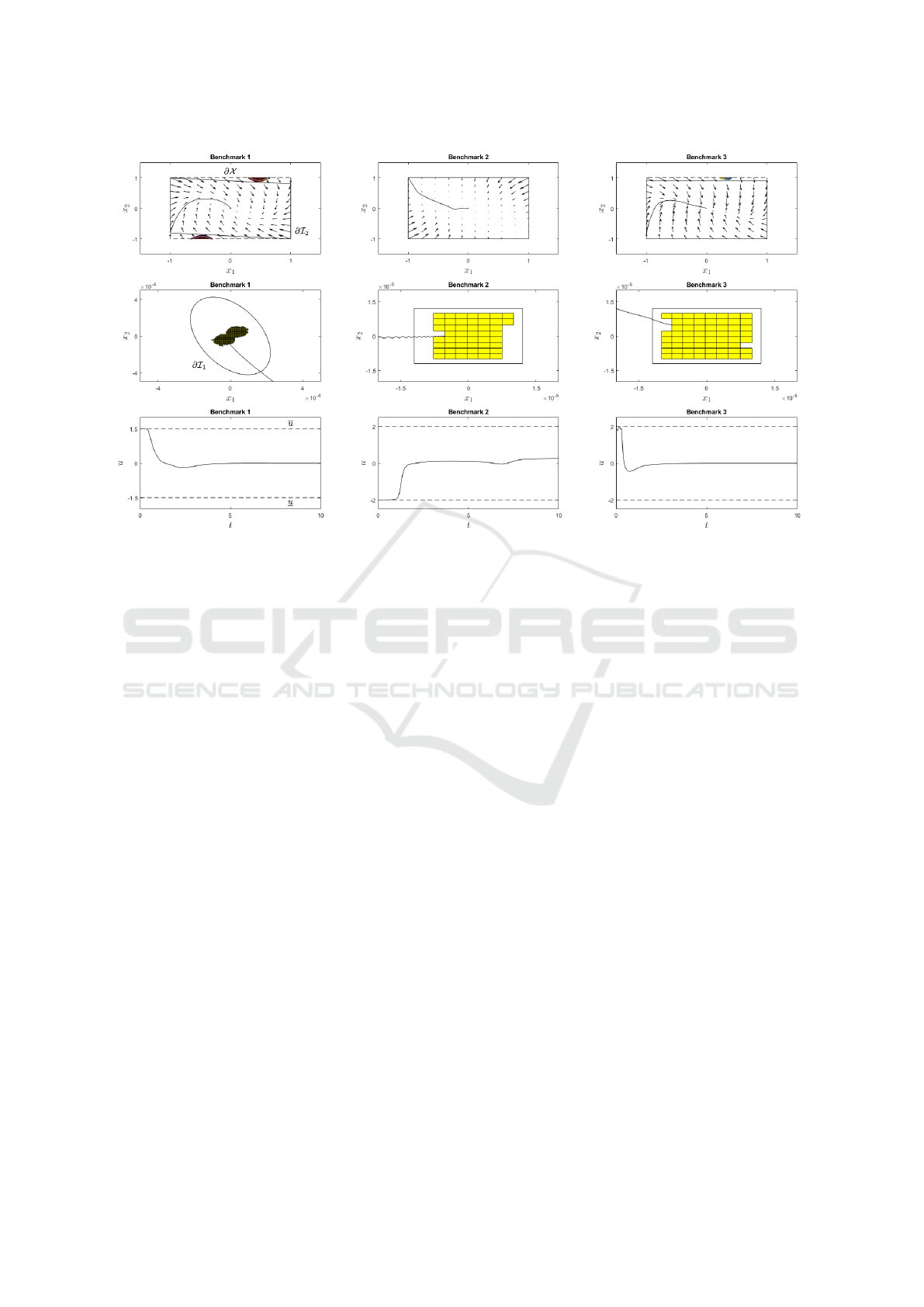
Figure 1: The ﬁgure shows the results obtained for the three benchmark problems, where the i-th column refers to Benchmark

i. The ﬁrst row illustrates the phase portraits of the closed-loop systems with the NN controllers. For each benchmark problem,

the boundary of X is illustrated by a dashed line, while a solid line is used to illustrate the boundary of I

, the set veriﬁed to

be positively invariant. Filled boxes show very small areas in which the derivative of the Lyapunov functions (determined by

use of Thm. 3) along the trajectories of the closed-loop systems could not be veriﬁed to be negative by interval arithmetics.

An enlarged version of the neighborhood of the origin is shown in the second row of ﬁgures: the boundary of the positively

invariant set I

⊂ I

is illustrated for each benchmark problem by a solid line. Since the Lyapunov function determined for

Benchmark i is strictly decreasing along the trajectories within Λ = I

\ I

, each state trajectory starting in I

reaches I

ﬁnite time, where it remains forever. This is shown for exemplary state trajectories, as well as for the corresponding input

trajectories in the third row of ﬁgures, showing that the input constraints (dashed lines) are satisﬁed.

6 CONCLUSION

This work has proposed a scheme for synthesizing

nonlinear controllers for nonlinear plants, such that

stabilization to an equilibrium point as well as the sat-

isfaction of input constraints is guaranteed. The con-

troller is established as NN controller with continu-

ous and continuously differentiable activation func-

tions in the units of its layers. By using sigmoid

functions as activation functions in the output layer,

the satisfaction of input constraints is ensured, even

if the same sigmoid functions are used in each unit.

A closed-form expression for the partial derivative of

the NN controller with respect to its input was de-

rived. Furthermore, insight was provided in how to

modify the bias vector in the output layer in order to

ensure that the origin is indeed an equilibrium point

of the closed-loop system. These aspects allow for

the use of Lyapunov’s indirect method in order to ver-

ify that the controlled system is asymptotically stable

with respect to the equilibrium point. For the case that

the veriﬁcation of asymptotic stability is successful, a

quadratic Lyapunov function can be found by solving

the Lyapunov equation for a selected positive deﬁnite

matrix. This has been used in the numerical examples

in order to verify safety and performance properties

with a software for reliable computations on the basis

of interval arithmetics. Future work addresses neces-

sary modiﬁcations for higher-dimensional spaces as

well as the investigation of other candidate Lyapunov

functions.

REFERENCES

Bellman, R. E. (1957). Dynamic Programming. Princeton

University Press.

Bertsekas, D. P. and Tsitsiklis, J. N. (1996). Neuro-dynamic

programming. Athena Scientiﬁc.

Blanchini, F. and Miani, S. (2008). Set-Theoretic Methods

in Control. Birkh

auser Boston.

Chang, Y.-C., Roohi, N., and Gao, S. (2020). Neural Lya-

punov Control. arXiv e-print:2005.00611.

Cybenko, G. (1989). Approximation by superpositions of a

ICINCO 2021 - 18th International Conference on Informatics in Control, Automation and Robotics

154

sigmoidal function. Mathematics of Control, Signals,

and Systems, 2(4):303–314.

Dutta, S., Chen, X., and Sankaranarayanan, S. (2019).

Reachability analysis for neural feedback systems us-

ing regressive polynomial rule inference. In Pro-

ceedings of the 22nd ACM International Conference

on Hybrid Systems: Computation and Control, pages

157–168.

Dutta, S., Jha, S., Sankaranarayanan, S., and Tiwari, A.

(2018). Output range analysis for deep feedforward

neural networks. In NASA Formal Methods, volume

10811 of Lecture Notes in Computer Science, pages

121–138. Springer International Publishing.

Fazlyab, M., Morari, M., and Pappas, G. J. (2020). Safety

veriﬁcation and robustness analysis of neural net-

works via quadratic constraints and semideﬁnite pro-

gramming. IEEE Transactions on Automatic Control

(early access). doi: 10.1109/TAC.2020.3046193.

Fazlyab, M., Robey, A., Hassani, H., Morari, M., and Pap-

pas, G. J. (2019). Efﬁcient and accurate estimation of

lipschitz constants for deep neural networks. In Ad-

vances in Neural Information processing Systems 32,

pages 11423–11434.

Goodfellow, I., Bengio, Y., and Courville, A. (2016). Deep

Learning. The MIT Press.

une, L. (2020). Computing Lyapunov functions using

deep neural networks. arXiv e-print:2005.08965.

Hagan, M. T. and Menhaj, M. B. (1994). Training feedfor-

ward networks with the marquardt algorithm. IEEE

Transactions on Neural Networks, 5(6):989–993.

Hornik, K., Stinchcombe, M., and White, H. (1989). Multi-

layer feedforward networks are universal approxima-

tors. Neural Networks, 2(5):359–366.

Hu, H., Fazlyab, M., Morari, M., and Pappas, G. J. (2020).

Reach-sdp: Reachability analysis of closed-loop sys-

tems with neural network controllers via semideﬁnite

programming. In 59th IEEE Conference on Decision

and Control, pages 5929–5934.

Huang, C., Fan, J., Li, W., Chen, X., and Zhu, Q. (2019).

Reachnn: Reachability analysis of neural-network

controlled systems. ACM Transactions on Embedded

Computing Systems, 18(5s):1–22.

Ivanov, R., Weimer, J., Alur, R., Pappas, G. J., and Lee,

I. (2019). Verisig: Verifying safety properties of hy-

brid systems with neural network controllers. In Pro-

ceedings of the 22nd ACM International Conference

on Hybrid Systems: Computation and Control, pages

169–178.

Khalil, H. K. (2002). Nonlinear systems. Prentice Hall.

Khalil, H. K. (2015). Nonlinear control. Pearson.

Kurakin, A., Goodfellow, I., and Bengio, S. (2016). Ad-

versarial examples in the physical world. arXiv e-

print:1607.02533.

Lewis, F. L. and Liu, D., editors (2013). Reinforcement

learning and approximate dynamic programming for

feedback control. IEEE Press and Wiley.

Liu, D., Wei, Q., Wang, D., Yang, X., and Li, H. (2017).

Adaptive Dynamic Programming with Applications in

Optimal Control. Springer International Publishing.

Markolf, L., Eilbrecht, J., and Stursberg, O. (2020). Tra-

jectory planning for autonomous vehicles combin-

ing nonlinear optimal control and supervised learning.

IFAC-PapersOnLine, 53(2):15608–15614.

Patterson, M. A. and Rao, A. V. (2014). Gpops-ii. ACM

Transactions on Mathematical Software, 41(1):1–37.

Perkins, T. J. and Barto, A. G. (2002). Lyapunov design

for safe reinforcement learning. Journal of Machine

Learning Research, 3:803–832.

Petridis, V. and Petridis, S. (2006). Construction of neu-

ral network based lyapunov functions. In The 2006

IEEE International Joint Conference on Neural Net-

work Proceedings, pages 5059–5065.

Richards, S. M., Berkenkamp, F., and Krause, A. (2018).

The lyapunov neural network: Adaptive stability cer-

tiﬁcation for safe learning of dynamical systems. In

Proceedings of The 2nd Conference on Robot Learn-

ing, volume 87, pages 466–476.

Rump, S. (1999). INTLAB - INTerval LABoratory. In

Csendes, T., editor, Developments in Reliable Com-

puting, pages 77–104. Kluwer Academic Publishers.

Sutton, R. S. and Barto, A. (2018). Reinforcement Learn-

ing: An Introduction. The MIT Press.

Stability Analysis for State Feedback Control Systems Established as Neural Networks with Input Constraints

155