A Comparative Study on Inﬂated and Dispersed Count Data

Monika Arora, Yash Kalyani and Shivam Shanker

Department of Mathematics, Indraprastha Institute of Information Technology, Delhi, India

Keywords:

Zero Inﬂated Data Regression Models, Dispersion, Machine Learning, Predictive Modeling.

Abstract:

The availability of zero inﬂated count data has led to the demonstration of various statistical models and

machine learning algorithms to be applied in diverse ﬁelds such as healthcare, economics and travel. However,

in real life there could be a count k > 0 that is inﬂated. There are only a few studies on k− inﬂated count

models. To the best of our knowledge, there is no article that demonstrates the machine learning algorithms

on such data sets. We apply existing k− inﬂated count models as well as machine learning algorithms on

travel data to compare the prediction and ﬁtness of the models and ﬁnd the signiﬁcant covariates. Our study

shows that the k− inﬂated models provide a good ﬁt to the data, however, the predictions from machine

learning algorithms are superior. This study can be extended further to include other artiﬁcial neural network

approaches on a larger data set.

1 INTRODUCTION

In many areas of study, a widely popular data type

explored is the count data. The Poisson distribution

is commonly used to study equi-dispersed count data.

The data is equi-dispersed when mean is equal to the

variance. In real life data sets, over-dispersion is a

common occurrence. The negative binomial distri-

bution is used when variance is more than mean or

over-dispersed in the count data. It is possible that

there is inﬂation at count zero for which the zero in-

ﬂated distributions are widely used. In seminal pa-

per, (Lambert, 1992) introduced zero inﬂated Poisson

(ZIP) regression model for zero inﬂated count data.

The ZIP regression models are applied in many areas

like life science (Ridout et al., 1998), (Hall, 2000),

travel (Lord et al., 2005), and economics (Gurmu and

Trivedi, 1996), (Cameron and Trivedi, 2013).

In the presence of over-dispersion in zero inﬂated

count data, zero inﬂated negative binomial (ZINB)

model is more appropriate and it was ﬁrst studied by

(Greene, 1994). Instead, of high frequency of zero it

is possible there is any count value k > 0 that is in-

ﬂated. The more appropriate choice for such data sets

is k−inﬂated count models. An extension of ZIP dis-

tribution is k−inﬂated Poisson (kIP) distribution. The

kIP model is a mixture of degenerate distribution at

k with probability π and Poisson (λ) with probabil-

ity (1 − π). It is a special case of zero and k inﬂated

Poisson (ZkIP) distribution studied by (Lin and Tsai,

2012) and (Arora, 2018). The kIP model is also a

special case of a k−inﬂated generalized Poisson dis-

tribution given by (Bae et al., 2005). The k−inﬂated

analog of negative binomial is k−inﬂated negative bi-

nomial (kINB) distribution. Recently, (Payandeh Na-

jafabadi and MohammadPour, 2018) studied kINB

for rate making system. As compared to zero inﬂated

count models, the literature on k−inﬂated count re-

gression models is not so rich.

The count regression models allow us to study the

the relationship between the response variables and

covariates. They allows us to ﬁnd signiﬁcant covari-

ates and make predictions. However, they have a few

limitations. They do not allow to study the non-linear

relationships of the covariates and are sensitive to out-

liers. There are various machine learning algorithms

that enable us to build a more robust and complex

regression models. They have good predictive abil-

ities and are efﬁcient. Recently, the approaches have

been applied on zero inﬂated count data (see (Lee and

Jin, 2006), (Arief and Murﬁ, 2018),(Alfredo et al.,

2018) ). Though, we did not come across any work

that demonstrates the machine learning algorithms on

k−inﬂated count data.

In this article, we consider the Poisson, NB and

their k−inﬂated analog regression models. We study

the ﬁt and prediction of the models using training and

test data, respectively. We perform 5-fold validation

and implement machine learning algorithms to make

the predictions. A comparative study between the

Arora, M., Kalyani, Y. and Shanker, S.

A Comparative Study on Inﬂated and Dispersed Count Data.

DOI: 10.5220/0010547700290038

In Proceedings of the 10th International Conference on Data Science, Technology and Applications (DATA 2021), pages 29-38

ISBN: 978-989-758-521-0

regression models and machine learning algorithms

show that the latter makes better predictions. The ar-

ticle is organized as follows. The Section 2 of the ar-

ticle describes statistical distributions and their corre-

sponding regression models. It also describes the ma-

chine learning algorithms applied in the article. We

demonstrate the methodology on a real life data set in

Section 3. A detailed analysis is performed in Sec-

tion 4. Lastly, Section 5 concludes the article.

2 METHODOLOGY

In this Section, we describe the methodologies used in

this article. We present the statistical distributions and

their regression models in Section 2.1 and Section 2.2,

respectively. The measures of ﬁt, described in Sec-

tion 2.3, are used to ﬁnd the best model. The machine

learning algorithms are described in Section 2.4. The

measures of prediction are given in Section 2.5.

2.1 Statistical Distributions

The Poisson and negative binomial are most com-

monly studied for count response variable. For

zero inﬂated count data, their zero inﬂated analogs,

zero inﬂated Poisson and zero inﬂated negative bi-

nomial are popular. While, for any count k >

0 their k−inﬂated analogs, k−inﬂated Poisson and

k−inﬂated negative binomial are more appropriate. In

this Section we brieﬂy describe Poisson, negative bi-

nomial and their k−inﬂated analogs.

Poisson Distribution. Let a response variable Y

follows a Poisson distribution with unknown parame-

ter λ > 0. The probability mass function (p.m.f.) of

random variable Y is given by

P(Y = y) =

−λ

; y = 0, 1,... . (1)

The mean and variance of Y is λ. It is the equi-

dispersion property of the distribution that makes it

popular. The other commonly used property of the

distribution is that it belongs to the exponential fam-

ily. Therefore, it is easy to ﬁnd the sufﬁcient statistics

and maximum likelihood estimates.

Negative Binomial Distribution. When the count

response is over-dispersed (variance>mean), then

negative binomial is a better choice. The p.m.f. of

a response variable Y from negative binomial distri-

bution is:

P(Y = y) =



y + θ − 1



(1 − p)

; y = 0, 1,. .. ,

(2)

where θ > 0 and 0 ≤ p ≤ 1.

k−Inﬂated Poisson Distribution. When zero is in

excess in count response, then zero inﬂated Poisson

(ZIP) distribution gives better ﬁt to the data. In real

life scenarios, any count k > 0 can be inﬂated. The

analogue distributions for such data sets is k− in-

ﬂated distributions. The k−inﬂated Poisson distribu-

tion (kIP) is a mixture of two distributions. One is

degenerate at k with probability π and the other is

Poisson (λ) with probability (1 − π). The p.m.f. of

a count response Y from kIP distribution is:

P(Y = y) =











π + (1 − π)

−λ

, y = k

(1 − π)

−λ

, y ≥ 0, y 6= k.

(3)

where 0 ≤ π ≤ 1 and λ > 0. When π = 0, (3) reduces

to Poisson distribution. The kIP distribution is a spe-

cial case of zero and k−inﬂated Poisson (ZkIP) dis-

tribution studied by (Lin and Tsai, 2012) and (Arora,

2018).

k− Inﬂated Negative Binomial Distribution. To

study the inﬂation at k > 0, the extension of NB dis-

tribution is k− inﬂated negative binomial (kINB) dis-

tribution. The p.m.f. of kINB is given by

P(Y = y) =







π + (1 − π)



k+θ−1



(1 − p)

, y = k

(1 − π)



y+θ−1



(1 − p)

, y 6= k.

(4)

On reparameterization, the variance of NB and kINB

models in R and SAS is given by Var(Y ) = λ + rλ

;

λ is the mean of response and r is the dispersion pa-

rameter. The high values of r corresponds to over-

dispersion in the data. When r is zero or close to zero,

it signiﬁes equi- or under-dispersion in the data.

2.2 Count Regression Models

To build the regression model, consider n indepen-

dent count responses Y = (Y

,. ..,Y

). The regres-

sion model corresponding to the Poisson distribu-

tion is popularly known as Poisson log linear regres-

sion model or simply a Poisson regression model.

The Poisson regression model is a generalized linear

model with a log link function. The Poisson regres-

sion model for the response vector Y is given by

log(λ

λ) = β

+ β

+ ... + β

. (5)

DATA 2021 - 10th International Conference on Data Science, Technology and Applications

where λ

λ = (λ

,. ..,λ

) is the rate parameter of the

model. The unknown parameters corresponding to

the vectors of covariates, x = (x

= 1, x

,. ..,x

) is

β = (β

,β

,. ..,β

). When the response variable fol-

lows a NB distribution then the NB regression model

is most appropriate. The link function in the NB re-

gression model can be obtained from (5) by replacing

λ by the mean of NB distribution.

The kIP model is constructed using the ZIP re-

gression model studied by (Lambert, 1992). The kIP

model links the covariates to the rate parameter λ

λ.

The inﬂation parameter π is linked to an unknown

constant using logit link. The model can be easily

extended to associate the desired covariates to the in-

ﬂation parameter π. The link functions are given by

log(λ

λ) = β

+ β

+ ... + β

logit(π) = γ. (6)

Similarly, the kINB regression model uses the same

link function as in kIP.

The Poisson, NB models and their k− inﬂated

analogs are implemented in SAS using GENMOD

and FMM procedures. The Poisson and NB models

are implemented in R using glm and glm.nb func-

tions, respectively. The kIP and kINB models are run

in R using optimization routine ’nlminb’. The routine

applies Newton-Raphson approach to obtain the esti-

mates. The algorithms in SAS and R use maximum

likelihood estimation approach to ﬁnd the estimates

of the unknown parameters. The results obtained in

SAS and R are same.

2.3 Hypothesis Testing and Model

Selection

In statistical modeling, hypothesis testing allows us to

study the signiﬁcance of the covariates. It also allows

to select a good ﬁt model. For the nested models, we

compare the models using likelihood ratio test (LRT).

Besides LRT, the popularly used measures to select a

good model are Akaike Information Criterion (AIC),

Bayesian Information Criterion (BIC) and R-squared.

The AIC and BIC are based on log-likelihood func-

tion of the corresponding model. In this Section, we

explain the hypothesis tests used to ﬁnd signiﬁcant co-

variates and unknown parameters in the Poisson, NB,

kIP and kINB models. We also describe the thumb

rule to choose best ﬁt model using AIC and BIC.

Hypothesis Testing. We use hypothesis testing to

study the signiﬁcance of the parameters. The hypoth-

esis H

: β

= 0 vs. H

: β

6= 0 tests the signiﬁcance

of the unknown jth covariate. The Wald test statis-

tic is z =

/SE(

). For large sample and under the

null hypothesis, the statistic approximately follows a

standard normal distribution.

The signiﬁcance of the dispersion parameters in

NB and kINB can also be tested. To test the dispersion

parameter r in NB and kINB models we use H

: r =

0 vs. H

: r 6= 0. The corresponding test statistic is

z = ˆr/SE(ˆr) ∼ N(0, 1).

The inﬂation parameter in the kIP and kINB mod-

els is 0 ≤ π ≤ 1. To test the signiﬁcance of inﬂation at

k, we test H

: π = 0 vs. H

: π > 0. Under the null, the

kIP and kINB models reduce to Poisson and NB, re-

spectively. Hence, the base models (Poisson and NB)

are nested in their k−analogs (kIP and kINB). For

nested models, we can perform LRT. The test statistic

is −2 logΛ = −2(L

−L

) where, L

is log-likelihood

of the model under null while L

is log-likelihood un-

der unrestricted. The test statistic follows a mixture of

distributions (Chant, 1974),(Shapiro, 1985). The

distribution of the test statistic changes as π = 0 is a

boundary point. Hence, the regularity conditions are

not met.

Akaike Information Criterion (AIC). There are

various measures that could be used to select the best

model. One of the most popular measures is AIC. It

is given by

AIC = −2 log L + 2p, (7)

where logL is the log-likelihood of the model and

p is the number of parameters in the model. The

measure is preferred as it prevents over ﬁtting of the

data. To prevent over ﬁtting it penalizes a model on

adding more parameters. The model with minimum

AIC gives the best ﬁt to the data. The difference be-

tween AIC of the various models is subjective. (Burn-

ham and Anderson, 2002) proposed a thumb rule for

AIC difference to choose the best model. The AIC

difference is given by

∆

= AIC

− min(AIC). (8)

Here, AIC

is AIC of ith model. The value of 0 ≤

∆

≤ 2 provides substantial support, 4 ≤ ∆

≤ 7 im-

plies considerably less support and ∆

> 10 essentially

provides no support for ith model.

Bayesian Information Criterion (BIC). Another

popular measure is the BIC. It is given by

BIC = −2 log L + p log n, (9)

where log L is the log-likelihood of the model, p is

the number of parameters in the model, and n is the

number of observations. It is also independent of the

prior and penalizes the model on its complexity. The

penalty term is larger in BIC than in AIC. While it has

A Comparative Study on Inﬂated and Dispersed Count Data

been commonly used for model identiﬁcation in lin-

ear regression and time series, it can, however, also be

applied to any set of maximum likelihood-based mod-

els (Schwarz, 1978). The model with minimum BIC

gives the best ﬁt to the data. As in the case of AIC,

there also exists a rule of thumb for model selection

based on BIC (Kass and Raftery, 1995).

∆

= BIC

− min(BIC). (10)

Here, BIC

is BIC of ith model. The value of ∆

can be

used as evidence against a candidate model to be the

best model. For 0 ≤ ∆

≤ 2, it is not worth more than

a bare mention, 2 < ∆

≤ 6, the evidence against the

model is positive, 6 < ∆

≤ 10, the evidence against

the model is strong, and ∆

> 10, the evidence against

the model is very strong.

2.4 Machine Learning Algorithms

In this Section, we describe the machine learning al-

gorithms applied in the study. The ﬁrst algorithm

we applied is decision trees. Decision Trees are one

of the most commonly used approaches in machine

learning. They help solve classiﬁcation as well as re-

gression problems. The algorithm constructs a tree

by breaking the dataset into smaller subsets and in-

crementally building the tree node by node. They are

easy to understand and interpret and require less ef-

fort for data preparation. Despite their advantages,

they are prone to overﬁtting and instability because of

their non-robustness. For categorical datasets, infor-

mation gain in decision trees are sometimes biased to

the attributes with more levels.

To obtain a better predictive performance than a

single model, ensemble methods like bagging and

boosting are typically used. Bagging (or Bootstrap

Aggregating) involves training the base model on ran-

dom subsets of the training dataset and then, aggre-

gating their results by either voting or averaging to

form a ﬁnal prediction. An example of this ensem-

ble method is random forests (RF), which uses this

technique along with feature bagging. The random

feature selection ensures that the trees are indepen-

dent of each other and provides a better performance

due to a better bias-variance trade-off. While bagging

involves ensemble voting, boosting involves sequen-

tially building an ensemble by training a new model

by re-weighting. The re-weighting involves adjusting

the weights of the samples which the previous model

has had highest error on. The recent algorithms that

demonstrate this technique are AdaBoost and XG-

Boost.

Random Forests. The random forests (RF) were

proposed by (Tin Kam Ho, 1995) and later extended

by (Breiman, 2001). They are considered to be one of

the most robust and accurate learning methods. The

technique is frequently used for both classiﬁcation

and regression. Using the concept of bagging, the al-

gorithm builds an ensemble of decision trees. Each

decision tree in the random forest provides a classiﬁ-

cation or prediction. By aggregating over the ensem-

ble, ﬁnal predictions are then made.

Over the last few years, signiﬁcant changes have

been made to increase the accuracy and overall per-

formance of the algorithm. The growth of these en-

sembles depends signiﬁcantly on the random vec-

tors used to grow each individual tree. (Breiman,

996b) suggested the use of bagging where each tree

is grown using a random selection (without replace-

ment) from the training set. (Dietterich, 2000) sug-

gested the use of random split selection, in which a

random split is selected at each node from among the

best m splits. (Tin Kam Ho, 1998) used the random

subspace method. It uses a random subset of features

to train every decision tree. Finally, (Breiman, 2001)

suggested the use of out-of-bag error to estimate the

generalization error.

Random Forests are still widely used due to their

numerous advantages. They are straightforward to ap-

ply and can be easily parallelized. They provide ac-

curacy as good as AdaBoost, even outperforming it

in some cases and is relatively robust to outliers and

noise. The various implementations of this algorithm

in languages like Python and R provide useful esti-

mates of error and variable importance.

Decision Trees. The decision trees are widely

known approach, commonly used for supervised

learning. They are majorly used for classiﬁcation

problems, but they could be used for regression analy-

sis as well. Similar to a tree, a decision tree comprises

of a root node, decision branches, interior nodes and

leaf nodes. The root node represents the initial node

or the most signiﬁcant feature. It could be used to

split the dataset into smaller subsets based on some

decision rules or choices from a number of alterna-

tives that are represented by the branches of the deci-

sion tree. The interior nodes and the leaf nodes rep-

resent intermediate features used for splitting and the

ﬁnal decision or outcome, respectively. There are var-

ious algorithms that could be used to build decision

trees such as Chi-squared Automatic Interaction De-

tection (CHAID), Classiﬁcation and Regression Trees

(CART), C5.0 and Quest, etc. In a decision tree, each

node may have two or more branches depending upon

the algorithm. The advantage of using decision tree

regression is that it requires very little bit of data pro-

cessing and it can capture nonlinear patterns easily. It

DATA 2021 - 10th International Conference on Data Science, Technology and Applications

is easy to interpret, understand and visualize. In this

article, we apply Decision Tree Regression (DTR).

Unlike the conventional decision trees which are used

for classiﬁcation, the DTR can predict numerical out-

comes of the dependent variables as well.

Adaptive Boosting. Adaptive Boosting or Ad-

aboost is one of the ﬁrst practical boosting methods

introduced by (Freund and Schapire, 1997). This al-

gorithm sequentially boosts weak learners to derive

an ensemble of strong learners which gives a bet-

ter prediction accuracy for the model. Similar to

RF, Adaboost is also an ensemble technique whose

baseline model is a decision tree. The weak learn-

ers are used in ensemble learning because a com-

plex function could be described by simpler general

trends which can provide a string approximation of

that function. Since, it is often difﬁcult to select an in-

dividual optimal learner from a variety of weak learn-

ers, boosting comes into play and simplify the selec-

tion process.

In Adaboost, weak learners are iteratively trained

on the training dataset by continual sampling with re-

placement. The predictive performance of the weak

learners is evaluated and the sampling distribution

weights are correspondingly updated for those sam-

ples which were incorrectly classiﬁed by this weak

learner. The next learner is trained on this resam-

pled distribution with updated weights. Adaboost was

initially introduced and widely used for classiﬁcation

problems, but it was also extended to regression anal-

ysis as well. The accuracy of the algorithm depends

majorly on the baseline model’s accuracy. It might

not give good results if the prediction hypothesis is

weak or sufﬁcient data is not available. We aim to in-

vestigate the prediction performance of Adaboost for

predicting numerical outcomes of the dependent vari-

able in comparison to other models.

Extreme Gradient Boosting. eXtreme Gradient

Boosting (or XGBoost) is an end-to-end scalable tree

boosting technique used for supervised learning. It

is an optimized implementation of gradient boosting

machines. It was introduced by (Chen and Guestrin,

2016). Due to its highly optimized algorithm and

system features, it is widely used by data scientists

around the world. The XGBoost algorithm itself im-

proves upon the gradient boosting machine frame-

work by reducing computational time and efﬁciently

allocating memory resources. It has sparse aware fea-

ture that handles missing values in the training data. It

also uses LASSO (L1) and Ridge (L2) regularization

to penalize the complexity of the model and comes

with built-in cross-validation while training. It imple-

ments the distributed weighted quantile sketch algo-

rithm to ﬁnd the optimum split points. Apart from

its algorithmic advantages, it also takes advantage of

the system to perform efﬁciently. It uses paralleliza-

tion, cache optimization, and out-of-core computing.

During training, it makes use of all CPU cores for

the construction of trees (parallelization). Its out-of-

core computing optimizes available disk space when

handling large datasets that do not ﬁt into memory.

Through cache awareness, it efﬁciently uses hardware

resources by allocating internal buffers in each thread

to store gradient statistics.

2.5 Prediction Analysis

The model selection is followed by model predic-

tion. The predictive power of the model ensures that

the model is robust to new observations. A popular

approach to study the model prediction is by con-

structing training and test data. The training data

is used to build the model. The best ﬁt model is

found using training data. The test data is used to

examine the prediction power of the best ﬁt model.

Here, for regression models the ratio of training to

test data is 80:20. We apply m-fold cross-validation

to the machine learning algorithms. There are various

measures to study the predictive performance of the

model. We use root mean square error and mean ab-

solute scaled error. The measures are based on com-

paring the error between observed and predicted re-

sponse.

m-fold Cross-validation. A m-fold cross validation

is a resampling procedure in which the dataset is split

into m smaller subsets known as folds. Using the

leave-one-out concept, one fold is left out for testing

while the model is trained on the remaining m-1 folds

in each iteration. This process is repeated for m itera-

tions in total and the aggregate result for the model is

derived by averaging over the results of each iteration.

The advantage of using m-fold cross-validation is that

it gives less biased and yet more accurate estimate by

reducing out-of-sample error.

Root Mean Square Error. The root mean squared

error (RMSE) is a commonly used measure. It is

given by RMSE=

∑

i=1

− ˆy

)

. Here, y

is the ob-

served count response and ˆy

is the predicted count re-

sponse for ith subject. The minimum value of RMSE

on test data indicates good predictive performance of

the model or machine learning algorithm under study.

A Comparative Study on Inﬂated and Dispersed Count Data

Mean Absolute Scaled Error. When there are zero

counts in the data, (Sellers and Shmueli, 2010) rec-

ommend to use mean absolute scaled error (MASE).

The MASE is given by mean



− ˆy

(1/n)

∑

i=1

− ¯y|



R-squared. The value of R-square (R

) is a good-

ness of ﬁt measure commonly used while assessing

the ﬁt of models. It is given by

∑

i=1

( ˆy

− ¯y)

∑

i=1

− ¯y)

, (11)

The value of R

is bounded between 0 and 1. The R

value of 1 indicates that the model perfectly ﬁts the

data.

3 DATA

To demonstrate the methodology we use a real life

data example. The data set is from Toronto Police

Service Public Safety data portal (Police, 2019). The

portal provides open access to the information on traf-

ﬁc collision in Toronto. The dataset consists of in-

formation on fatal and non-fatal; pedestrian and non

pedestrian accidents. It has information on the type

of vehicles involved in the accident, namely, automo-

biles, cyclist, motorcyclists, emergency vehicles and

trucks. Similar data sets have been considered in nu-

merous studies (see (Lord et al., 2005),(Lord et al.,

2008)).

We considered data on non-fatal accidents of non

pedestrians accidents from year 2013-2019. In the

database, each accident is identiﬁed by a unique ac-

cident number (or ACCNUM). The ACCNUM is the

same for the people involved in an accident. On the

basis of ACCNUM we extracted information on the

number of non-fatal injured people. In this study, we

predict the number of non-fatal injuries (NoNonFa-

tal) for non pedestrian accidents. The response vari-

able, ’number of non-fatal injuries’ (NoNonFatal) is

a count response. It takes values from 0 to 13. There

are various covariates in the database, but, many of

them have missing observations. On the basis of rel-

evance and data availability, we choose the number

of people injured or involved in an accident (NoIn-

jured), light, cyclist, automobile, truck, motorcycle,

emergency vehicle and transit or city vehicle (Trsnci-

tyveh) as covariates in the study. The ’NoInjured’ is a

discrete count variable. The environmental covariate

light has 9 categories so it was treated as a continu-

ous variable. The categories of the light covariate are

dark, daylight, dark and artiﬁcial, dawn, dusk, dusk

and artiﬁcial, daylight and artiﬁcial, dawn and arti-

ﬁcial, other. The other covariates have binary cate-

gories yes or no so they are considered as categorical

covariates.

4 ANALYSIS

We demonstrate the methodologies discussed in Sec-

tion 2 on a real life data set. The data set is brieﬂy

described in Section 3. The response variable is num-

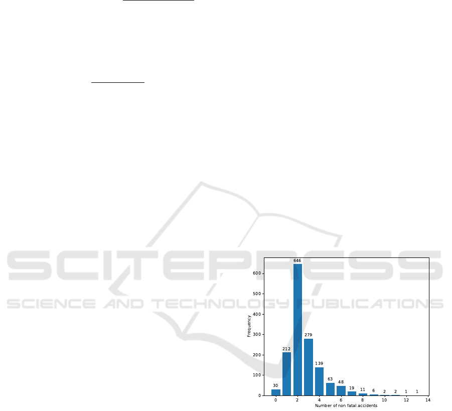
ber of non-fatal injuries (NoNonFatal) in an accident.

After removing possible outliers and missing obser-

vations there are 1459 independent subjects and 8

covariates in the study. The mean and variance of

the count response are 2.63 and 2.46, respectively.

The frequency at count 2 is 646 (44.28%). The pre-

liminary analysis shows that the data is possibly, al-

most equi-dispersed or slightly under-dispersed and

inﬂated at k = 2. The histogram and boxplot of the

response variable are shown in Figures 1 and 2, re-

spectively. The correlation analysis on the covariates

did not show any strong correlation. Thus, all the co-

variates mentioned in Section 3 are included in the

study.

Figure 1: Histogram of response.

The count regression models described in Section 2.2

are built to study the relationship between response

variable and covariates. The statistical models are

also used to make the predictions. To perform the

analysis the data is divided into training (80%) and

test (20%) data. The training data set is used to con-

struct and ﬁnd the best model. While, the test data is

used to make the predictions. In the training data, the

response variable has mean 2.63 and variance is 2.51.

The mean and variance of test data are 2.65 and 2.30,

respectively. The frequency of 2 in the training data is

499 (42.76%) while the frequency of 2 in the test data

is 147 (50.34%). The descriptive analysis shows that

DATA 2021 - 10th International Conference on Data Science, Technology and Applications

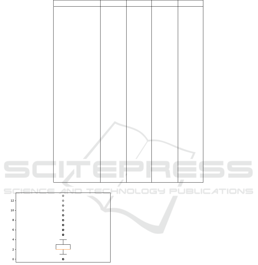
Table 1: Estimates, standard errors (in parentheses) and model diagnostics (log-likelihood, AIC) for the training data.

Parameter kINB kIP NB Poisson

Intercept 0.4984* 0.4984* 0.4568* 0.4568*

(0.2894) (0.2894) (0.2725) (0.2725)

NoInjured 0.2433* 0.2433* 0.2444* 0.2444*

(0.0087) (0.0087) (0.0083) (0.0083)

Light 0.0071 0.0071 0.0060 0.0060

(0.0124) (0.0124) (0.0113) (0.0113)

Cyclist -0.0623 -0.0623 -0.0475 -0.0475

(0.0567) (0.0567) (0.0487) (0.0487)

Automobile -0.2640* -0.2640* -0.2006* -0.2006*

(0.0920) (0.0920) (0.0799) (0.0799)

Truck -0.0376 -0.0376 -0.0331 -0.0331

(0.0879) (0.0879) (0.0801) (0.0801)

Motorcycle -0.0135 -0.0134 -0.0081 -0.0081

(0.0600) (0.0600) (0.0534) (0.0534)

Emergency Vehicle -0.1144 -0.1144 -0.1091 -0.1091

(0.2260) (0.2260) (0.2151) (0.2151)

Trsncityveh -0.0886 -0.0886 -0.0805 -0.0805

(0.0885) (0.0885) (0.0826) (0.0826)

γ -1.2777 -1.2778 – –

(0.1163) (0.1163)

ˆr < 0.0001 – < 0.0001 –

– –

π 0.2179* 0.2179* – –

(0.0198) (0.0198)

No. of parameters 11 10 10 9

Log-likelihood -1620.70 -1620.70 -1689.06 -1689.06

AIC 3261.40 3261.40 3398.12 3396.12

BIC 3312.00 3312.00 3441.70 3441.70

Figure 2: Boxplot of the response.

the training and test data has high frequency at 2. A

small positive difference between mean and variance

is preserved which indicates the existence of almost

equi-dispersion or a slight under-dispersion.

The high frequency of 2 in the training data in-

dicates inﬂation at k =2. Thus, we construct kINB,

kIP, NB and Poisson regression models. The parame-

ter estimates and their standard errors (in parentheses)

are given in Table 1. The signiﬁcant parameters at

10% level of signiﬁcance are asterisk marked. From

Table 1, it could be observed that NoInjured and Au-

tomobile are signiﬁcant covariates in all the models

considered under study. The intercept is signiﬁcant

at 10% level while other parameters are signiﬁcant at

5% level of signiﬁcance as well.

The Table 1 shows that Poisson is a parsimonious

model as it has least number of parameters. While,

NB and kIP have equal number of parameters. The

kINB has 11 parameters, thus is the most complex

model in the study. The kIP and kINB models have

signiﬁcant inﬂation at 5% level of signiﬁcance with

π = 0.2179. The estimated value of the dispersion

parameter (ˆr) in NB and kINB models is < 0.0001.

When the data is under- or equi-dispersed then the

NB model might not converge. On convergence it

is reduced to the Poisson model. Here, the nega-

tive binomial (NB) model did not converge in SAS

and R. Thus, it gives identical results to the Poisson

model. While, the kINB model is reduced to the kIP

model. The data is almost equi-dispersed, hence, NB

and kINB models are reduced to Poisson and kIP, re-

spectively.

To ﬁnd the best model, we use LRT, AIC and

BIC as described in Section 2.3. The AIC and BIC

difference between Poisson and kIP model is 134.72

A Comparative Study on Inﬂated and Dispersed Count Data

Table 2: Comparison of statistical models on training data with signiﬁcant parameters.

Parameter kINB kIP NB Poisson

Intercept 0.2219* 0.2218* 0.2131* 0.2131*

(0.0399) (0.0399) (0.0353) (0.0353)

NoInjured 0.2431* 0.2431* 0.2441* 0.2441*

(0.0083) (0.0083) (0.0079) (0.0079)

Automobile -0.2194* -0.2196 * -0.1611* -0.1611*

(0.0825) (0.0826) (0.0699) ( 0.0699)

γ -1.2795* -1.2794* – –

(0.1164) (0.1164)

ˆr < 0.0001 – < 0.0001 –

– –

π 0.7824* 0.7824* – –

No. of parameters 5 4 4 3

Log-likelihood -1622.10 -1622.10 -1690.31 -1690.31

AIC 3252.20 3252.20 3388.62 3386.62

BIC 3272.50 3272.50 3408.86 3401.80

Table 3: Predictive performance of the statistical models on training and test data with all the covariates.

Train Test

Measure kINB kIP NB Poisson kINB kIP NB Poisson

RMSE 0.7919 0.7919 0.8578 0.8578 0.6932 0.6932 0.8172 0.8172

MASE – – – – 0.3840 0.3840 0.3400 0.3400

(>> 10) and 129.7 (>> 10), respectively. The kINB

is reduced to the kIP model and has same AIC and

BIC as kIP model. The NB model did not converge

and the AIC of NB (3398.12) is slightly higher than

the Poisson (3396.12) model. Based on the thumb

rule given by (Burnham and Anderson, 2002) and

(Kass and Raftery, 1995), the kIP model is best ﬁt

for the data. The Poisson and kIP models are nested

so we can apply the LRT. The hypothesis is H

: π = 0

vs. H

: π > 0. The LRT statistic is −2logΛ =136.72

with p− value < 0.0001 and H

gets rejected. Equiva-

lently, inﬂation at k =2 is signiﬁcant. Here, the NB did

not converge in R and SAS. When the data is under-

or equi-dispersed then the NB is reduced to Poisson

irrespective of convergence. On performing LRT on

NB and kINB models, we get exactly same results.

So, kINB has signiﬁcant inﬂation at k=2.

We re-ran the models with only signiﬁcant covari-

ates, see Table 2. All the parameters are signiﬁcant

at 5% level of signiﬁcance. We get the similar inter-

pretations. The kIP and kINB models perform better

than their base (Poisson and NB) models. The inﬂa-

tion at k=2 is signiﬁcant in both the kIP and kINB

models. We observe from Table 1 and 2 that the co-

variate NoInjured has a positive impact on the mean

response, while, automobile has a negative impact.

We compared the predictive performance of the

models on the test data. The RMSE values of the test

and training data of kINB, kIP, NB and Poisson mod-

els are given in Table 3. The RMSE value of kINB

and kIP models is same for the test and training data.

Similarly, the RMSE value of NB and Poisson mod-

els are 0.8172 and 0.8578 for test and training data,

respectively. The RMSE of kINB and kIP models is

less than that of NB and Poisson models for both, test

and training data. On comparing the NB and Poisson

models to their k−inﬂated analogs we obtain MASE

of 0.3840 for kINB and kIP models. While, for NB

and Poisson we get MASE equal to 0.3400. The less

RMSE and MASE on test data implies less error in

prediction and hence better predictive powers. There-

fore, kINB and kIP models have slightly less predic-

tion error than their base counterparts.

The data science models like random forests and

XGBoost are popularly used for predictions. To make

the predictions on the count response, we use tech-

niques described in Section 2.4. We apply decision

trees, random forests, Adaboost and XGBoost on the

training dataset using cross-validation. In the decision

trees we apply decision tree regression (DTR) analy-

sis which essentially uses the CART algorithm. Here,

for cross validations we used ﬁve-folds. The predic-

tions are made on test data. The RMSE and MASE

are calculated to evaluate the performance of the ma-

chine learning algorithms. The scikit-learn library of

Python is used to perform the analysis.

In the training data, apart from AdaBoost all the

algorithms have RMSE ∼ 0.34. The RMSE of de-

DATA 2021 - 10th International Conference on Data Science, Technology and Applications

Table 4: Predictive performance and goodness of ﬁt of the machine learning algorithms (Decision Trees (DT), Random Forests

(RF), Adaptive Boosting (AdaBoost), eXtreme Gradient Boosting (XGBoost) on training and test data with all the covariates.

Train Test

Measure DT RF AdaBoost XGBoost DT RF AdaBoost XGBoost

RMSE 0.3406 0.3424 0.3866 0.3420 0.3814 0. 3748 0.4238 0.3698

MASE – – – – 0.1225 0.1181 0.1578 0.1150

0.9617 0.9610 0.9410 0.9611 0.9468 0.9489 0.9252 0.9495

Table 5: Comparison of feature importance using machine learning algorithms.

Parameter Decision Trees Random Forests AdaBoost XGBoost

NoInjured 0.9930 0.9906 0.9878 0.9784

Light 0.0031 0.0041 0.0062 0.0029

Cyclist 0.0010 0.0011 0.0013 0.0079

Automobile 0.0005 0.0010 0.0008 0.0018

Truck 0.0006 0.0010 0.0009 0.0032

Motorcycle 0.0005 0.0010 0.0013 0.0027

Emergency Vehicle < 0.0001 < 0.0001 < 0.0001 0.0004

Trsncityveh 0.0009 0.0009 0.0013 0.0024

cision trees is minimum (0.3406) and the RMSE of

random forests and XGBoost are very close. The

AdaBoost has slightly higher RMSE than random

forests. Further, the machine learning algorithms are

run on the test data. We observe, XGBoost has low-

est RMSE (0.3698) while, the AdaBoost has the high-

est RMSE (0.4238). The random forests perform bet-

ter than decision trees with a decrease of 1.73% in

RMSE. On comparing random forests to XGBoost

we observe an improvement of 1.33%. The XGBoost

shows a signiﬁcant decrease of 3.04% when com-

pared to decision trees.

The average MASE is determined by evaluating

the average of MASE values obtained using ﬁve-fold

validation. According to MASE measure, the least

value is of the XGBoost (0.1150). While, the highest

is of AdaBoost (0.1578). From Table 4, we observe

that there is slight improvement in the predictions as

we go from decision trees to random forests. Simi-

larly, XGBoost performs better than random forests.

To study the ﬁt of the machine learning algorithms we

study R

values of the training and test data. From Ta-

ble 4, we observe that the XGBoost provides the best

goodness of ﬁt with an R

of 0.9611 and 0.9495 for

training and test data, respectively. The R

of decision

trees, random forests and XGBoost are approximately

close, while, AdaBoost provides slightly poor ﬁt. Ad-

ditionly, from Table 5, we observe that ’NoInjured’

is the most important feature to predict the response.

The feature is signiﬁcant in the statistical models as

well (see Table 1).

In conclusion, from the preliminary analysis we

observe that the training data is almost equi-dispersed

or slightly under-dispersed and inﬂated at k = 2. Us-

ing AIC, BIC and LRT, kIP model is the most appro-

priate model for the data set. On the basis of predic-

tion measures kIP and kINB performs equally well. It

is observed that the data is almost equi-dispersed thus

kINB is reduced to kIP model. The kIP model is par-

simonious. Thus, kIP model is the best choice for the

data set. While we have used parametric approaches

via statistical modeling to build a model and make

predictions, we also aim to study the non-parametric

approaches provided by the machine learning algo-

rithms. Using R

as the goodness of ﬁt measure and

RMSE and MASE as predictive indicators on vari-

ous machine learning algorithms, we observe that as

expected XGBoost performed best. Notably, the deci-

sion trees which do not involve any ensemble methods

performed poor as compared to the ensemble models

but signiﬁcantly better than the statistical models.

5 SUMMARY

While, there are many studies on zero inﬂated count

data there are only a few applications shown on

k−inﬂated count data. In real life data sets, the occur-

rence of k > 0 inﬂated count data is not insigniﬁcant.

We demonstrate the application of k−inﬂated count

models. When there is inﬂation at k and data is equi-

dispersed, k−inﬂated Poisson is the most appropriate

model. We observe that the statistical models provide

a good ﬁt and decent predictions. However, the pre-

dictions obtained using machine learning algorithms

are considerably better. The machine learning algo-

rithms are easy to apply and the computational time

is very less. The complexity of the machine learn-

A Comparative Study on Inﬂated and Dispersed Count Data

ing algorithms make them difﬁcult to comprehend.

Although, the algorithms provide information on the

importance of the covariates; they do not provide any

information on the direction (positive or negative) of

contribution in the model. Thus, to study k−inﬂated

count data sets, the corresponding regression mod-

els are appropriate for interpretations while, machine

learning algorithms give superior predictions. So, it is

recommended to study both the approaches. Our fu-

ture work involves studying the approach on a larger

data set from a different area. We plan to extend the

comparative study by including various artiﬁcial neu-

ral network approaches.

REFERENCES

Alfredo, S. G., Dutang, C., and Petrini, L. (2018). Machine

learning methods to perform pricing optimization. a

comparison with standard glms. Variance, Casualty

Actuarial Society.

Arief, F. M. and Murﬁ, H. (2018). The accuracy of xgboost

for insurance claim prediction. International Journal

of Advances in Soft Computing and Its Applications.

Arora, M. (2018). Extended Poisson models for count data

with inﬂated frequencies. PhD thesis, Old Dominion

University.

Bae, S., Famoye, F., Wulu, J., Bartolucci, A., and Singh,

K. (2005). A rich family of generalized poisson re-

gression models with applications. Mathematics and

Computers in Simulation, 69(1):4–11. Second Special

Issue: Selected Papers of the MSSANZ/IMACS 15th

Biennial Conference on Modelling and Simulation.

Breiman, L. (1996b). Out-of-bag estimation. Technical re-

port, Department of Statistics, University of Califor-

nia, Berkeley.

Breiman, L. (2001). Random forests. Machine Learning,

45(1):5–32.

Burnham, K. P. and Anderson, D. R. (2002). Model Selec-

tion and Multimodel Inference. Springer.

Cameron, A. C. and Trivedi, P. K. (2013). Regression Anal-

ysis of Count Data. Cambridge Press, London, UK.

Chant, D. (1974). On asymptotic tests of composite

hypotheses in nonstandard conditions. Biometrika,

61:291–298.

Chen, T. and Guestrin, C. (2016). Xgboost: A scal-

able tree boosting system. Proceedings of the 22nd

ACM SIGKDD International Conference on Knowl-

edge Discovery and Data Mining.

Dietterich, T. G. (2000). An experimental comparison of

three methods for constructing ensembles of decision

trees: Bagging, boosting, and randomization. Ma-

chine Learning, 40(2):139–157.

Freund, Y. and Schapire, R. E. (1997). A decision-theoretic

generalization of on-line learning and an application

to boosting. Journal of Computer and System Sci-

ences, 55(1):119–139.

Greene, W. (1994). Accounting for excess zeros and sam-

ple selection in Poisson and negative binomial regres-

sion models. Working papers, New York University,

Leonard N. Stern School of Business, Department of

Economics.

Gurmu, S. and Trivedi, P. (1996). Excess zeros in count

models for recreational trips. Journal of Business &

Economic Statistics, 14(4):469–477.

Hall, D. B. (2000). Zero-inﬂated Poisson and binomial re-

gression with random effects: A case study. Biomet-

rics, 56:1030–1039.

Kass, R. E. and Raftery, A. E. (1995). Bayes fac-

tors. Journal of the American Statistical Association,

90(430):773–795.

Lambert, D. (1992). Zero-inﬂated Poisson regression, with

an application to defects in manufacturing. Techno-

metrics, 34:1–14.

Lee, S.-K. and Jin, S. (2006). Decision tree approaches for

zero-inﬂated count data. Journal of Applied Statistics,

33(8):853–865.

Lin, T. H. and Tsai, M.-H. (2012). Modeling health survey

data with excessive zero and k responses. Statistics in

Medicine, 32:1572–1583.

Lord, D., Guikema, S. D., and Geedipally, S. R. (2008).

Application of the Conway-Maxwell-Poisson general-

ized linear model for analyzing motor vehicle crashes.

Accident Analysis & Prevention, 40:1123 – 1134.

Lord, D., Washington, S. P., and Ivan, J. N. (2005). Poisson,

poisson-gamma and zero-inﬂated regression models

of motor vehicle crashes: balancing statistical ﬁt and

theory. Accident Analysis & Prevention, 37(1):35 –

46.

Payandeh Najafabadi, A. T. and MohammadPour, S. (2018).

A k-inﬂated negative binomial mixture regression

model: Application to rate–making systems. Asia-

Paciﬁc Journal of Risk and Insurance, 12(2).

Police, T. (2019). Toronto police service public safety data

portal. website.

Ridout, M., Demetrio, C., and Hinde, J. (1998). Models for

count data with many zeros. In International Biomet-

ric Conference, Cape Town.

Schwarz, G. (1978). Estimating the dimension of a model.

The Annals of Statistics, 6(2):461–464.

Sellers, K. F. and Shmueli, G. (2010). Predict-

ing censored count data with COM-Poisson re-

gression. Technical report, Robert H. Smith

School Research Paper No. RHS-06-129. Avail-

able at SSRN: https://ssrn.com/abstract=1702845 or

http://dx.doi.org/10.2139/ssrn.1702845.

Shapiro, A. (1985). Asymptotic distribution of test statistics

in the analysis of moment structures under inequality

constraints. Biometrika, 72:133–144.

Tin Kam Ho (1995). Random decision forests. In Pro-

ceedings of 3rd International Conference on Docu-

ment Analysis and Recognition, volume 1, pages 278–

282 vol.1.

Tin Kam Ho (1998). The random subspace method for con-

structing decision forests. IEEE Transactions on Pat-

tern Analysis and Machine Intelligence, 20(8):832–

844.

DATA 2021 - 10th International Conference on Data Science, Technology and Applications