VDNA-Lab: A Computational Simulation Platform for DNA

Multi-strand Dynamics

Frankie Spencer

1 a

, Usman Sanwal

1 b

and Eugen Czeizler

1,2 c

Department of Information Technologies,

Abo Akademi University, Turku, Finland

National Institute for Research and Development of Biological Sciences, Bucharest, Romania

Keywords:

DNA Assembly Simulator, Multi-strand Assembly, Rule-based Modeling, Graphical User Interface,

Course-grained Modeling.

Abstract:

The dynamics of nucleic-acids dynamical systems is intrinsically based on local interaction. The major acting

mechanisms are that of Watson-Crick complementarity on one-hand, generating binding events, and ther-

mal energy on the other, generating random motion and un-binding. It is thus predictable that such systems

can be successfully captured by computational modeling paradigms based on local interactions, such as the

rule-based modeling methodology. In this research we introduce the Virtual DNA Lab (VDNA-Lab) a sim-

ulation tool which provides an easy to use graphical interface for creating, running and visualizing synthetic

simulations for DNA assembly systems, such as assembly of DNA nanostructures, strand displacement cas-

cades systems, DNA-tile assembly etc. It employs a custom designed model, implemented in the BioNetGen

Language (BNGL) formalism, to capture the DNA dynamics, as well as the NFsim computational model-

ing engine to run simulations and generate outputs. These outputs can be visualized using the VDNA-Lab’s

own visualization tool, which allows also for further analysis and ﬁltering. The software is freely available at

https://github.com/Frankie-Spencer/virtual dna lab.

1 INTRODUCTION

The fast increase of computational power experienced

in the past decade has made it possible for computer

scientists to develop various modeling and simula-

tion techniques giving them access to very high levels

of details for various self-assembly phenomena, de-

spite that achieving such levels is prohibitively expen-

sive in real experiments. Thus, the use of computer

simulations in the ﬁeld of self-assembly is now well

accepted as well as its role in better understanding

of many quantitative details of such systems(Thomas

and Schwartz, 2017), (Kamerlin and Warshel, 2011),

(Glotzer et al., 2004). A major challenge for the mod-

eling of self-assembly biological phenomena lies in

the fact that we have to deal with an extremely large

space of possible assembly pathways accessible to the

intermediate species of a self-assembly reaction net-

work. Another challenge arises from the fact that

self-assembly reactions are sensitive to many physical

constrains (e.g. structural, chemical) available within

https://orcid.org/0000-0002-6775-1832

https://orcid.org/0000-0002-2178-3329

https://orcid.org/0000-0002-1607-1554

the original in vivo environment, conditions which

are hard to be replicated within the in silico computa-

tional models (Ariga and et al., 2008). Despite these

challenges there are a variety of modeling methods

available such as SSA/Gillespie approaches (Sweeney

and et al., 2008), (Blinov and et al., 2004) or Rule-

based approaches (Mohammed et al., 2017), (Danos

and et al., 2009), which have been proven valuable for

the study and analysis of self-assembly systems.

Nanotechnology is one of the leading worldwide

undertakings of the scientiﬁc community. Within this

ﬁeld, DNA has proved itself as a very powerful and

versatile construction material(Kuzyk et al., 2009),

(Li and et al., 2011) and (Lund and et al., 2010).

Recent advances in DNA-based nanotechnology have

opened the way towards the systematic engineering

of inexpensive nanoscale devices for a multitude of

purposes (Krishnan and Simmel, 2011), (Li and et al.,

2011), (Lund and et al., 2010). Self-assembly prop-

erties of DNA, which are based on speciﬁc and pre-

dictable Watson-Crick based pairing rules, make it a

highly malleable and controllable nanomaterial (See-

man, 2003).

There are several tools available for modeling and

288

Spencer, F., Sanwal, U. and Czeizler, E.

VDNA-Lab: A Computational Simulation Platform for DNA Multi-strand Dynamics.

DOI: 10.5220/0010546302880294

In Proceedings of the 11th International Conference on Simulation and Modeling Methodologies, Technologies and Applications (SIMULTECH 2021), pages 288-294

ISBN: 978-989-758-528-9

visualization of complex DNA-based self-assembly

constructions. These tools include the Visual DSD

(DNA Strand Displacement) tool (Lakin and et al.,

2011), focused on modeling DNA strand displace-

ment reaction systems, Iowa State University Tile As-

sembly Simulator (ISU TAS) (Patitz, 2011), focused

on modeling DNA-tile assembly, or oxDNA (Popple-

ton and et al., 2020), which is a course grained mod-

eling tool for the physical atom-level simulation of

DNA assembly systems. Rule-based modeling ap-

proaches have also been used for modeling the ki-

netics of DNA-based Tile Assembly Systems (Mo-

hammed et al., 2017), as well as for DNA strand dis-

placement cascades (Gautam. et al., 2020).

In our work, we provide a framework for rule-

based modeling of generalized DNA multi-strand dy-

namics, where DNA molecules and their interac-

tions are modeled at nucleotide level. We have used

the BioNetGen Language (BNGL) formalism (Blinov

and et al., 2004) and the NFsim computational plat-

form (Sneddon and et al., 2011) as well as a com-

prehensive collection of aiding (Python) subroutines

which facilitate the user interface and make the mod-

eling experience available for the user without having

any prior knowledge of the BNGL modeling frame-

work. In order to track and report global mapping

of the components within a heterogeneous complex,

we have developed a visualization interface, details

provided in Section 3, which not only helps to vi-

sualize the results but also can be used for further

numerical analysis. The software is freely available,

see (Spencer et al., 2021).

2 MATERIAL AND METHODS

2.1 Rule-based Modeling

Modeling and simulation of self-assembly biochemi-

cal systems is a challenging computational task, as the

modeler has to deal with both a high combinatorial

number of species, namely all the generated partial-

and sub-assemblies, and also with a large numbers

of reactions between these species. The Rule-based

modeling approach, which employs the idea of sub-

dividing molecules, or generally species-entities, into

their primary components, denoting protein domains,

active sites or any other feature of the particle, can

be used to solve this problem (Faeder et al., 2009).

Within the rule-based modeling paradigm, molecules

are represented as agents with a ﬁnite number of inde-

pendent sites. The sites provide the agent-agent bind-

ing functionality and as a result molecular complexes

are generated. Rules are only deﬁned on the basis of

local patterns which provide a compact representa-

tion about agents’ interaction. In rule-based model-

ing, models are deﬁned in terms of a speciﬁc syntax

(rules) instead of writing the model mathematically

directly. After that a semantic is presented in order to

cover the differences between what is written and the

mathematical deﬁnition of its computation. A care-

fully described syntax increases the model’s accessi-

bility for domain experts that are not familiar with the

modeling and mathematical formalisms (Faeder et al.,

2009).

Two useful simulation tools for rule-based mod-

eling are BioNetGen (Faeder et al., 2009) and NF-

sim (Sneddon and et al., 2011). BioNetGen is a

BNGL-compatible simulation tool that implements

various indirect methods including both determin-

istic and stochastic methods. NFsim is also a

BNGL-compatible simulation tool that implements a

(stochastic) direct method which applies a speciﬁc

network-free simulation and thus avoids enumeration

of species and reactions, that may be intractable for

large models (Yang and Hlavacek, 2011). There are

six different blocks of a BNGL ﬁle, namely: param-

eters, species, observables, molecule types, reaction

rules and functions. Further detail about these blocks

and NFSim simulator can be found in (Faeder et al.,

2009) and (Sneddon and et al., 2011).

2.2 A Computational Modeling

Framework for DNA Multi-strand

Dynamics

We have created a generic computational modeling

framework for DNA multi-strand dynamics using the

BioNetGen Language (BNGL) formalism and the

NFsim computational platform. The DNA molecules

and the subsequent interactions are captured starting

from nucleotide level. Each nucleotide (as a bio-

entity) is represented as an individual instance of a

generic agent N (from nucleotide) which has 1 state-

characteristic site, b (from base), and 3 connecting

sites: 5’, 3’, and W. Relating to its biological coun-

terpart, the site b can be in exactly one of the four

possible states: A (Adenine), G (Guanine), C (Cyto-

sine), or T (Thymine); moreover, once initialized, site

b will never change its state. The remaining sites of

agent N are used for connecting the nucleotide within

the single-stranded molecule it is part of

, i.e., us-

DNA is composed primarily of nucleotides with a sugar-

phosphate backbone; the nucleotides are attached to the

backbone to form a structure which is known as a single-

stranded DNA (ssDNA) molecule. The ssDNA is repre-

sented with two different ends. By convention, one end of

the backbone is know as the 5’ end and the second one is

VDNA-Lab: A Computational Simulation Platform for DNA Multi-strand Dynamics

289

ing sites 5’ and 3’, and for connecting the nucleotide

with a complementary base-pair

, using site W. For

example, within our rule-based model, the basic struc-

ture for the single-stranded DNA (ssDNA) molecule

ATTGCTA is shown in Figure 1.

Figure 1: The schematic representation of the ssDNA com-

plex ATTGCTA within our BNGL model.

VDNA-Lab takes as input populations of isolated

(5’-to-3’ oriented) single-stranded DNA molecules

(ssDNAs) and simulates their binding and dissocia-

tion reactions. At the core of this model implemen-

tation lie 12 binding and un-binding local interaction

rules, each with its own kinetic rate constant, and each

implemented through one or several rule-based reac-

tions. Using these reactions/rules, we capture the dy-

namics of the DNA-dynamical system, by modeling:

• the initial binding of short toeholds, i.e., short

complementary sequences of 3-to-7 nucleotides;

• the ”breathing” dynamics in-between bounded ss-

DNAs, i.e. zipping and unzipping reactions;

• random un-binding events (between one pair of

nucleotides);

• the un-binding of loosely connected ssDNAs.

The list of all rule-types and their associated ki-

netic rate constants is presented in Table 1. By de-

fault, VDNA-Lab provides some normalized values

for these kinetic rate constants, see the 4-th column

of the table. However, any of these values can be up-

dated by the user using the Advanced option.

3 RESULTS: THE VDNA-Lab

SOFTWARE

We have developed the VDNA-Lab (Virtual DNA

Lab) software to provide an easy to use graphical in-

terface for creating, running and visualizing synthetic

simulations for DNA assembly systems, such as as-

sembly of DNA nanostructures, strand displacement

cascades systems, DNA-tile assembly etc. It uses the

NFsim computational modeling engine to run simu-

lations and generate outputs. These outputs can be

visualized using the VDNA-Lab’s visualization tool,

known as the 3’ end.

The base-pair nucleotides A-T and C-G are complemen-

tary which means their shape allows them to bond together

with hydrogen bonds.

which allows also some further analysis of the simu-

lation output. Here we explain the different features

and parameters of the VDNA-Lab software.

The tool consists of three main functionalities,

each reachable from a speciﬁc tab on the upper left

corner of the main window:

• Create Test Tube for creating new test tube input

ﬁles; these are called also species ﬁles, as they are

stored on computer with the extension .species

• Run Experiment for simulating the assembly pro-

cess within a given input test tube ﬁle, and

• Visualize Test Tube for visualizing the content of

a test tube at the beginning, middle, or end of an

experiment.

The Create Test Tube feature of VDNA-Lab, see

Fig. 2 is used to create/edit new species ﬁles, to be

used as input in the Run Experiment process. ssDNA

sequences are entered by the user (only strings over

A,T,C and G are allowed to be entered as input) in

the Desired ssDNA sequence tab and the number of

copies of the generated ssDNA structure has to be in-

troduced in the Amount tab (by default 1 copy is cre-

ated). Once the user presses the Add button, these

sequences are added to the List of ssDNA to be cre-

ated text box. After the ssDNA sequences are cre-

ated, the user can Edit, Delete, or Reset all of them.

The user can also import the ssDNA sequences, or

even more complicated multi-ssDNA complexes, us-

ing the Import from Species button on the right hand

side. Such species ﬁles can be extracted for exam-

ple from the default output ﬁles generated during the

numerical simulation phase, i.e., from the ”Run ex-

periment” tab. Thus, the user can select the input

single complementary bases

The two interacting ssDNA segments can be part of the

same ssDNA molecule, i.e., a hairpin loop, or be two dis-

tinct ssDNA molecules bound within the same complex.

That is, both ssDNA strands continue with pairwise non-

bounded sequences to one direction -at least one strand

should not be bound to anything else- and bound sequences

of length at least 1 to the other direction

There are several cases within the model where two nu-

cleotides become/remain bounded, although such a situa-

tion might not occur experimentally. These situations are:

i) single complementary bases in the middle of two non-

complementary (or non-bound) ssDNA sequences; ii) sin-

gle complementary base positioned at the end of a non-

complementary (or not-bound) sequence; iii) single com-

plementary base, where the complement is on the same

ssDNA, at distance 0 or 1; iv) single complementary base

when the opposite neighbors of the pair are bound but not

complementary, i.e., are bound but not to each-other

The default value of the kinetic rate constant K

max

imple-

menting an instantaneous reaction is set to 10

SIMULTECH 2021 - 11th International Conference on Simulation and Modeling Methodologies, Technologies and Applications

290

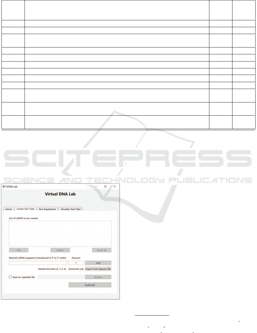
Table 1: The list of 12 rules governing the dynamics of the DNA self-assembly process, and the default values of their

associated kinetic rate constants. The kinetic rate constants are scaled according to the rate of the intra-complex toehold

binding of complementary segments, i.e., Rule 4, which is normalized to value 1.

Rule# Description of rule action kinetic

param.

(k.p.)

default

val. of

k.p.

Rule 1 toehold binding of compl. seq. (3-to-7 bases) of 2 un-connected ssDNA k

0.001

Rule 2 binding of s.c.b.

of two immediately-connected ssDNA segments

300

Rule 3 binding of s.c.b. of two closely-connected (1-off neighbor connection) ssDNA

segments

Rule 4 toehold binding of compl. seq. (3-to-7 bases) of two connected ssDNA k

Rule 5 un-binding of s.c.b. positioned at a split

Rule 6 un-binding of s.c.b. positioned in the middle of a compl. sequence k

0.1

Rule 7 un-binding of s.c.b. where at least one ssDNA ends on that position k

Rule 8 very rapid (instantaneous) un-binding between s.c.b. in abnormal conditions

max

Rule 9 random unbinding of a pair of bound nucleotides k

0.01

Rule

rapid un-binding of a size-2 comp. seq. in the middle of non-compl./non-bound

seq.

300

Rule

rapid un-binding of a size-3 comp. seq. in the middle of non-compl./non-bound

seq.

100

Rule

rapid un-binding of a size-4 comp. seq. in the middle of non-compl./non-bound

seq.

sequences of an experiment to be the output multi-

ssDNA structures generated during previous simula-

tions. Moreover, the newly generated input ﬁle can be

saved as a new species ﬁle, using the ”Save as custom

species ﬁle” check-box, or it will become (by default)

the current test tube to be simulated.

Figure 2: The Create Test Tube environment for creat-

ing/editing test tube (.species) ﬁles.

The Run Experiment feature, see Fig. 3 is used to

numerically simulate the DNA assembly process from

a given input .species ﬁle, or (by default) from the cur-

rent test tube. The VDNA-Lab software uses NFsim

simulator on background to run experiments. NFsim

needs several parameters to run and produce output

(.dump) ﬁles for a certain simulation. The user can

enter numerical values for the Start time, Number of

dumps and Sim. end (i.e., end model-time for the sim-

ulation); the default values for these entries are 0, 10,

and 1, respectively. The output, i.e., .dump, ﬁles are

saved within a newly created folder, named after the

name of the input ﬁle and the time of the simulation;

the location of this folder is introduced by the user

using the Save simulation output directory tab.

The Run Experiment feature has also several Ad-

vanced options. By selecting this tab, a new win-

dow opens giving the user advanced choices regard-

ing three modeling aspects, each contained within a

delimited area of the window:

First, the user can select between using the default

BNGL model ﬁle

, describing the entire model’s en-

tities and all their interaction rules, or a separate user-

speciﬁed .bngl model ﬁle, possibly describing a user-

altered variant of this model; such possible model-

variant modiﬁcations are suggested with respect to

the custom temperature-controlled annealing proto-

cols detailed below.

The default BNGL model ﬁle is called master VDNA-

LAB BNGL model.bngl, and it is placed within the folder

... \system ﬁles\

reference ﬁles of the VDNA-Lab instal-

lation folder

VDNA-Lab: A Computational Simulation Platform for DNA Multi-strand Dynamics

291

Figure 3: The Run simulation environment.

The second advanced feature offers the possibility

to modify the kinetic rate constants of the 12 reaction

rules indicated in Table 1, which are governing the

entire assembly (and dis-assembly) dynamics.

Finally, the third advanced feature allows the

user to deﬁne an annealing protocol for the simu-

lation/experiment, during which the temperature of

the system, and subsequently part of the reaction

rates, are modiﬁed several times mid simulation.

Namely, the user can specify the start and end tem-

perature of the system, the (constant) temperature

decrease/increase per annealing step, as well as the

length of time each annealing step will last. By de-

fault, without the annealing mechanism, the system

is assumed at a (normalized) temperature Temp =

1. When the annealing mechanism is activated, the

kinetic rate constants of reaction rules 5–12, from

within Table 1, are multiplied by the Temp values,

while the kinetic rate constants of reaction rules 1–

4 remain unmodiﬁed. If the user wants to create new

Temp-dependable kinetic rate constants for any of the

above rules, then he can modify the default BNGL

model ﬁle

within the ”begin functions ... end func-

tions” block, and then select the option of using this

custom .bngl model ﬁle.

The Visualize Test Tube window, see Fig. 4, can

be used by the user to generate a browser-based text-

enhanced visualization of the content of a simulation

output (.dump) ﬁle, see e.g. the visualization from

Fig. 5 associated to the running example discussed in

the next section. Within the visualization, each com-

plex, composed from one or several bound ssDNA,

is displayed separately, with each ssDNA within the

complex on a separate line. Per each ssDNA we rep-

Figure 4: The Visualized Test Tube environment.

resent the nucleotide sequence, either on the 5’ to 3’

order, or on the reverse order. The ﬁrst ssDNA of

a complex is always displayed on the 5’ to 3’ or-

der, while subsequent ssDNAs within the complex

have the reversed order of the ﬁrst complemented se-

quence. Moreover, if some particular nucleotide is

bound to another, by hovering the mouse over this

nucleotide its complement will highlight too. Also,

consecutive segments of bound nucleotides will have

a similar coloring. Due to these features, the user can

easily see the active domains of the complex, i.e., se-

quences of consecutive nucleotides bound to comple-

mentary contiguous sequences.

The Advanced option gives user further ability to

obtain ﬁltered results, highlights, and also get stats

about the selected ﬁltered complexes. Further details

made available by the visualization feature will be de-

scribed below, when we provide a running example of

our software on several simple input instances.

3.1 Running Examples

In this section, we present two running examples for

our computational simulation platform, one designed

to capture a DNA strand-displacement reaction, and

the other following the assembly of DAE-E DNA-

tiles (Jiang and et al., 2017). In both cases, VDNA-

Lab takes as input populations of isolated (or partially

bounded) oriented ssDNAs, and simulates their bind-

ing and dissociation reactions. The kinetic rate con-

stants used within these examples are the software de-

fault values, which means that the rates are normal-

ized and thus the current model-time is different from

what one might observe in a real wet-lab experiment.

SIMULTECH 2021 - 11th International Conference on Simulation and Modeling Methodologies, Technologies and Applications

292

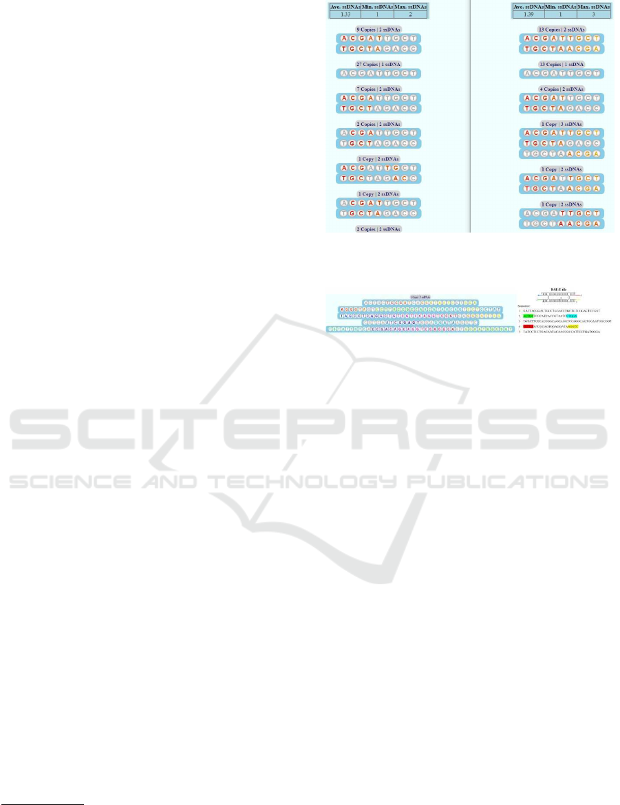
In our ﬁrst test case, for the ﬁrst simulation, we

introduced 20 copies ot the ssDNAs:

ACGAT T GCT and CCAGATCGT

We simulated the assembly for 0.1 second (model-

time), and we visualize the content of the test-tube,

see Fig. 5 a) for a fraction of this visualization

On top of the visualization window, we display

some basic statistics providing the content of the test-

tube, namely the average, minimum and maximum

number of ssDNAs per complex. For example, for

our test-tube visualization in Fig. 5 a) we have that

the average number of ssDNAs per complex is 1.33,

while the minimum and maximum numbers of ss-

DNA within a complex are 1 and 2, respectively.

Within a visualization window, each distinct con-

ﬁguration corresponding to a complex is visualized

only once. However, within a given test-tube (i.e.,

conﬁguration) there could be many identical copies

of the same complex. In such a case, the amount of

identical copies are summed up and mentioned ac-

cordingly on top of each complex, as well as the num-

ber of ssDNAs that are included in that complex. For

example, regarding the ﬁrst visualized complex from

Fig. 5 a) we can say that within that test-tube there are

9 complexes having the exactly same conﬁguration.

Single ssDNA within a complex can be identiﬁed as

a chain of nucleotides placed on consecutive position.

Multiple ssDNAs within a complex appear each on

a separate line. The nucleotides that are bound to

a complementary pair appear in color, whereas non-

complemented nucleotides are displayed in gray. Mi-

nor color shift can be noticed within nucleotides that

are consecutively complemented or that are closely

located in an ssDNA.

Continuing our example, after the initial assem-

bly, using the Import from Species function from the

Create Test Tube window we add to the current con-

ﬁguration 20 copies of the new ssDNA

AGCAATCGT

The simulation is restarted for another 0.5 seconds,

after which the output is visualized in Fig. 5 b)

As it can be observed from Fig. 5 b), one can ob-

serve both the situations were a strand displacement is

in process, for those complexes containing 3 ssDNA

molecules, and situations in which one of the initially

bounded ssDNA molecules has been completely dis-

placed, and only the two fully complementary strands

are either partial or completely bound.

The entire content of the test tube and thus of the visual-

ization window requires more space, and thus was omitted

As before, due to space limitation only a fraction of the

visualization window is displayed

Figure 5: Fraction of simulation output after 0.1s and sub-

sequent 0.5s after addition of new ssDNA.

Figure 6: Generated output of a DNA self-assembly system

simulation and the desired layout of a DAE-E DNA-tile.

In a completely different experiment we have cre-

ated a test-tube containing 20 copies of each of the 5

ssDNA molecules forming a DAE-E DNA-tile (Jiang

and et al., 2017). We have simulated their assembly

for 1 second and then visualized the output. In Fig. 6

we display one of the visualized complexes consist-

ing of 5 ssDNA bound together into a successfully as-

sembled DAE-E tile, as well as the desired schematic

representation of such a tile.

4 CONCLUSIONS

In this paper, we have introduced VDNA-

Lab (Spencer et al., 2021), a computational modeling

framework for DNA multi-strand dynamics using the

BioNetGen Language (BNGL) formalism (Harris,

2015) and the NFsim computational platform (Sned-

don and et al., 2011). The ssDNAs are provided as

input while the system simulates their binding and

dissociation reactions. The model implementation

is done with the help of 12 binding and un-binding

local interaction rules. Each of these rules has its

own, user-adjustable, kinetic rate constant and each

of them is implemented through one or several rule-

based reactions. Tracking and reporting the global

mapping of the components within a heterogeneous

complex is done with the help of a VDNA-Lab visu-

alization subroutine. The content of the dynamical

system is unloaded at various time-points within the

VDNA-Lab: A Computational Simulation Platform for DNA Multi-strand Dynamics

293

simulation, and it is re-assembled for visualization

and further numerical analysis. A simple 2D graphi-

cal representation of the assembled complexes is also

generated, where one can track the ssDNAs within

the complex as well as all the binding interactions.

Different from other computational modeling

frameworks for DNA strand assembly, we can modify

some of the systems parameters, such as the temper-

ature of the system, during the system simulation.

Thus, we can model also an entire annealing process

for the formation of a DNA structure. The underlining

computational modeling engine used by VDNA-Lab,

namely NFsim, allows also for other parameters to be

adjusted mid-simulation: e.g., we can deﬁne speciﬁc

binding/un-binding kinetic rates for each different

length-3 subsequence. Currently, VDNA-Lab does

not have these features implemented.

ACKNOWLEDGEMENTS

This work was partially supported by the Academy of

Finland, project 311371/2017, and by the Romanian

National Authority for Scientiﬁc Research and Inno-

vation, PED grant 2391.

REFERENCES

Ariga, K. and et al. (2008). Challenges and breakthroughs

in recent research on self-assembly. Science and Tech-

nology of Advanced Materials, 9(1):014109.

Blinov, M. L. and et al. (2004). BioNetGen: software for

rule-based modeling of signal transduction based on

the interactions of molecular domains. Bioinformat-

ics, 20(17):3289–3291.

Danos, V. and et al. (2009). Rule-based modelling and

model perturbation. In Transactions on Computa-

tional Systems Biology XI, pages 116–137. Springer.

Faeder, J. R., Blinov, M. L., and Hlavacek, W. S. (2009).

Rule-Based Modeling of Biochemical Systems with

BioNetGen, pages 113–167. Humana Press, NJ.

Gautam., V., Long., S., and Orponen., P. (2020). Ruledsd:

A rule-based modelling and simulation tool for dna

strand displacement systems. In Proceedings of the

13th International Joint Conference on Biomedical

Engineering Systems and Technologies - Volume 3:

BIOINFORMATICS,, pages 158–167.

Glotzer, S. C., Solomon, M. J., and Kotov, N. A. (2004).

Self-assembly: From nanoscale to microscale col-

loids. AIChE Journal, 50(12):2978–2985.

Harris, L. A. e. a. (2015). BioNetGen 2.2: Advances

in Rule-Based Modeling. arXiv e-prints, page

arXiv:1507.03572.

Jiang, S. and et al. (2017). Understanding the elemen-

tary steps in dna tile-based self-assembly. ACS Nano,

11(9):9370–9381.

Kamerlin, S. C. L. and Warshel, A. (2011). Multiscale

modeling of biological functions. Phys. Chem. Chem.

Phys., 13:10401–10411.

Krishnan, Y. and Simmel, F. C. (2011). Nucleic acid based

molecular devices. Angewandte Chemie International

Edition, 50(14):3124–3156.

Kuzyk, A., Laitinen, K. T., and T

orm

a, P. (2009). DNA

origami as a nanoscale template for protein assembly.

Nanotechnology, 20(23):235305.

Lakin, M. R. and et al. (2011). Visual dsd: a design

and analysis tool for dna strand displacement systems.

Bioinformatics, 27:3211–3213.

Li, J. and et al. (2011). Self-assembled multivalent dna

nanostructures for noninvasive intracellular delivery

of immunostimulatory cpg oligonucleotides. ACS

Nano, 5(11):8783–9.

Lund, K. and et al. (2010). Molecular robots guided by

prescriptive landscapes. Nature, 465(7295):206–209.

Mohammed, A., Czeizler, E., and Czeizler, E. (2017).

Computational modelling of the kinetic tile assembly

model using a rule-based approach. Theoretical Com-

puter Science, 701:203 – 215. At the intersection of

computer science with biology, chemistry and physics

- In Memory of Solomon Marcus.

Patitz, M. J. (2011). Simulation of self-assembly in the

abstract tile assembly model with ISU TAS. CoRR,

abs/1101.5151.

Poppleton, E. and et al. (2020). Design, optimization and

analysis of large DNA and RNA nanostruc through in-

teractive visualization, editing and molecular simula-

tion. Nucleic Acids Research, 48(12):e72–e72.

Seeman, N. (2003). Dna in a material world. Nature Cell

Biology, 421(6921):427–431.

Sneddon, M. and et al. (2011). Efﬁcient modeling, simula-

tion and coarse-graining of biological complexity with

nfsim. Nat Methods, 8(2):177–183.

Spencer, F., Sanwal, U., and Czeizler, E. (2021). VDNA-

Lab. Available at https://github.com/Frankie-Spencer/

/virtual dna lab , version 1.0.

Sweeney, B. and et al. (2008). Exploring the parameter

space of complex self-assembly through virus capsid

models. Biophysical Journal, 94(3):772 – 783.

Thomas, M. and Schwartz, R. (2017). Quantitative compu-

tational models of molecular self-assembly in systems

biology. Physical Biology, 14(3):035003.

Yang, J. and Hlavacek, W. S. (2011). The efﬁciency of

reactant site sampling in network-free simulation of

rule-based models for biochemical systems. Physical

Biology, 8(5):055009.

SIMULTECH 2021 - 11th International Conference on Simulation and Modeling Methodologies, Technologies and Applications

294