Sustainable Development Goals Monitoring and Forecasting using Time

Series Analysis

Yassir Alharbi

1,3 a

, Daniel Arribas-Bel

2 b

and Frans Coenen

1 c

Department of Computer Science, The University of Liverpool, Liverpool L69 3BX, U.K.

Department of Geography and Planning, The University of Liverpool, Liverpool L69 3BX, U.K.

Almahd College, Taibah University, Al-Madinah Al-Munawarah, Saudi Arabia

Keywords:

Time Series Causality, Missing Values, Hierarchical Classiﬁcation, Time Series Forecasting, Sustainable

Development Goals.

Abstract:

A framework for UN Sustainability for Development Goal (SDG) attainment prediction is presented, the

SDG Track, Trace & Forecast (SDG-TTF) framework. Unlike previous SDG attainment frameworks, SDG-

TTF takes into account the potential for causal relationship between SDG indicators both with respect to the

geographic entity under consideration (intra-entity), and neighbouring geographic entities to the current entity

(inter-entity). The challenge is in the discovery of such causal relationships. Six alternatives mechanisms are

considered. The identiﬁed relationships are used to build multivariate time series prediction models which

feed into a bottom-up SDG prediction taxonomy, which in turn is used to make SDG attainment predictions.

The framework is fully described and evaluated. The evaluation demonstrates that the SDG-TTF framework

is able to produce better predictions than alternative models which do not take into consideration the potential

for intra and inter- causal relationships.

1 INTRODUCTION

Time series forecasting is a signiﬁcant task under-

taken within the context of many application domains

such as budget planning (Deschamps, 2004), weather

forecasting (Qing and Niu, ). The fundamental build-

ing block of time series forecasting is to use the time

series past lags to predict single or multiple time steps

ahead(Jason, 2018). The complexity of time series

analysis increases in the presence of short time se-

ries, the number of missing values, and unevenly dis-

tributed time series. This paper examines the appli-

cation of time series analysis to Sustainable Develop-

ment Goal (SDG)(UN, 2559) attainment forecasting,

progress tracking and tracing. The challenges can be

summarised as follows: (i) the short time series to be

utilised (maximum of 20 observations); (ii) the noisy

nature of the data, which also features a lot of miss-

ing values, and which therefore needs an intensive

amount of preprocessing and interpolation, (iii) the

hierarchical nature of the data (geographical location

https://orcid.org/0000-0001-6764-030X

https://orcid.org/0000-0002-6274-1619

https://orcid.org/0000-0003-1026-6649

→ goal → target → indicator → . . . ), (iv) the lack

of speciﬁc attainment values (thresholds) and (v) the

computational complexity of causal inference in the

context of the short SDG time series data.

In (Alharbi et al., 2019) an SDG prediction frame-

work, the SDG Attainment Prediction (SDG-AP)

framework, was presented to answer basic questions

regarding SDG attainment, such as “will geographi-

cal entity x reach it is SDG goals by 2030?”. The

model assumed that each time series was independent

of every other time series; that there was no intra-

entity relationship between SDG time series within

the same geographic entity (region, country), and no

inter-regional relationship between SDG time series

across entities (regions, countries). Each time series

was considered in a univariate manner. The predic-

tion model was founded on a bottom-up hierarchical

taxonomy and classiﬁcation framework; a framework

incorporated into subsequent work.

In (Alharbi et al., 2020), an alternative framework

was presented, the SDG Correlated Attainment Pre-

diction (SDG-CAP) framework. The framework was

founded on the same hierarchical framework as used

in (Alharbi et al., 2019), but took into consideration

the intra-entity relationship between the various SDG

Alharbi, Y., Arribas-Bel, D. and Coenen, F.

Sustainable Development Goals Monitoring and Forecasting using Time Series Analysis.

DOI: 10.5220/0010546101230131

In Proceedings of the 2nd International Conference on Deep Learning Theory and Applications (DeLTA 2021), pages 123-131

ISBN: 978-989-758-526-5

123

time series in a single geographic entity; the pos-

sibility that there might be inter-entity relationships

between the SDG time series in neighbouring geo-

graphic entities was not considered. A multivariate

time series analysis approach was adopted. To iden-

tify relationships between time series within a sin-

gle geographic entity ﬁve different “ﬁltration” mech-

anisms (causal relationship discovery mechanisms)

were considered. It was found that by combining the

results of all ﬁve ﬁltration mechanisms, referred to as

the ACA mechanism after the authors, a best perfor-

mance was achieved, out-performing SDG-AP.

In this paper we present the SDG Multivariate

Track, Trace and Forecast (SDG-TTF) framework

that takes into consideration both intra-entity rela-

tionships and inter-geographic region causalities be-

tween SDGs. The proposed SDG-TTF model in-

corporates the hierarchical framework from (Alharbi

et al., 2019), and the ACA causality relationship

mechanism from (Alharbi et al., 2020) for intra-

and inter-entity relationship discovery. The proposed

SDG-TTF framework enhances forecasting effective-

ness compared to previous approaches.

The rest of this paper is organised as follows. In

the following section, Section 2, a brief literature re-

view of relevant work underpinning the work pre-

sented in this paper is given. The SDG application

domain and the SDG time series data set is described

in Section 3. The required preparation of the SDG

data is then considered in Section 4. The proposed

SDG-TTF approach is described in Section 5 and its

evaluation in Section 6. A case study describing the

System operation is given in Section in 7 .The paper

concludes with a summary of the main ﬁndings, and a

number of proposed directions for future research, in

Section 8.

2 LITERATURE REVIEW

The proposed SDG-TTF approach addresses two fun-

damental challenges: (i) short time series forecasting

and (ii) time series causal inference. Previous work in

these two areas is therefore considered in the ﬁrst two

sub-sections in this literature review. The literature

review is completed with some discussion of previous

work directed at SDG forecasting.

2.1 Short Time Series Forecasting

Short time series forecasting is challenging because it

is difﬁcult to perform meaningful out of sample eval-

uation, or cross validation, given the low number of

observations (Hyndman and Kostenko, 2007). From

the literature a range of methods have been proposed

to address this issue, see for example (De Gooijer and

Hyndman, 2006). However, these proposed solutions

still insist on 50 or more observations. In the case of

the SDG data, the sample size is less than 20 points.

The FBProphet time series forecasting tool was used

in (Alharbi et al., 2019) for the purpose of SDG at-

tainment prediction where it was demonstrated that

FBProphet produced a better prediction accuracy over

two alternatives, ARMA and ARIMA. FBProhpet de-

compose a time series y into three parts, trend (g),

seasonality (s) and holiday (h), plus an error term ε,

as shown in Equation 1.

y = g + s + h + ε (1)

FBProhpet is a uni-variate predictor; given that the

focus of this paper is prediction using sets of causal-

related time series a multi-variate approach is re-

quired. A multivariate time series forecasting model,

using Long Short Term Memory (LSTM) networks,

was presented in (Jason, 2018). The LSTM model

demonstrated a better overall performance compared

two alternatives, namely ARMA and ARIMA (De

Gooijer and Hyndman, 2006). The LSTM model

was adopted in (Alharbi et al., 2020) for multi-variate

SDG attainment forecasting. More generally, LSTM

models have been widely adopted with respect to

many real-life applications such as weather (Qing and

Niu, ) and stock market(Chen et al., 2015) predic-

tion. With respect to the work presented in this paper

an Encoder-Decoder LSTM, was used (Jason, 2018).

LSTM typically performs better when large data sets

are used. But also seems to perform well when a large

number of short time series are used in a multi-variate

setting.

2.2 Time Series Causal Inference

Causal inference is concerned with the process of

establishing a connection (or the lack of a con-

nection) between events or instances. Given two

candidate time series, A = {a

, a

, . . . , a

} and B =

, b

, . . . , b

}, where wish to establish that B is

causality-related to A, this is typically established

using a prediction mechanism that uses the “lag”

, . . . , b

m−1

} to predict a

. We then compare the

predicted value for a

with the known value, for ex-

ample using the Root Mean Square Error (RMSE)

measure. If the two values are close then that “time

series A is causality-related to time series B”.

There are a number of mechanisms that can be

adopted to achieves the above. With respect to the

work presented in this paper six such mechanisms

are considered for evaluation purposes: (i) Granger

DeLTA 2021 - 2nd International Conference on Deep Learning Theory and Applications

124

Causality (GC), (ii) the Temporal Causal Discov-

ery Framework (TCDF), (iii) Pearson coefﬁcient, (iv)

Lasso, (v) the Mann-Whitney U Test. and (vi) ACA.

Each is considered in further detail below.

2.2.1 Granger Causality

Granger Causality (GC) is one of the most widely

used causal inference mechanisms found in the liter-

ature (Narayan and Smyth, 2009; D

orgo et al., 2018).

It was introduced in the 60s and is calculated as shown

in Equation 2 where: (i) X and Y are time series, (ii)

a and b are the laggs of X and Y , (iii) t is the current

time step and (iv) e is a residual error. The idea is that

if time series X “granger cause” time series Y , then the

past values of X should contain helpful information to

forecast X in a manner that would be better than when

forecasting X without historical data. The variation

of GC that was used with respect to the research pre-

sented in this paper is Stats-models variation (Seabold

and Perktold, 2010). GC has been used previously in

the context of SDG prediction, for example in (D

orgo

et al., 2018) 20,000 pairs of time series that featured

causal relationship were found.

Xt = a

t−1

+ b

t−1

+ e (2)

2.2.2 Temporal Causal Discovery Framework

The Temporal Causal Discovery Framework (TCDF)

(Nauta et al., ) is an alternative mechanism to deter-

mine whether a time series A has a caused association

with a time series B. TCDF uses a Convolutional Neu-

ral Network (CNN) whose internal parameters are in-

terpreted to discover causal relations. The framework

has been shown to not work well with respect to short

time series (for best performance it is suggested that

1000 data points are required, but is still used for eval-

uation purposes in this paper.

2.2.3 Pearson Correlation

Pearson Correlation (Frey, 2018) has been used to

measure the correlations between any given pair of

time series. The mechanism assumes linearity of the

data. This assumptions holds with respect to many

SDG time series that are typically linearly spaced,

2.2.4 Lasso

Lasso (Tibshirani, 1996) is an L1 regularisation tech-

nique frequently used to reduce high dimensionality

data, which can also be employed to establish the

existence of a causality between variable (Epprecht

et al., 2013; Tibshirani, 1996). LASSO reduces the

dimensionality of the input data set by penalising vari-

ances to zero, thus allowing irrelevant variables to be

removed. Equation 3 shows the LASSO cost func-

tion. Inspection of the equation indicates that the ﬁrst

part is the squared error function, whilst the second

part is a penalty applied to the regression slope. If λ is

equal to 0, then the function becomes a normal regres-

sion. However, if λ is not 0 coefﬁcients are penalised

accordingly, leaving only coefﬁcients that can explain

the variance in the data.

L C F =

∑

i=1

−

∑

i j

+ λ

∑

j=1



(3)

2.2.5 Mann-Whitney U Test

The Mann-Whitney U Test (Alam and Rudin, 2015)

is the ﬁfth causal inference mechanism used in this

paper. The test is used to determine if any two pairs

of time series are statistically different. It is a non-

parametric test (unlike, for example, Lasso).

2.2.6 ACA

The last of the six causality discovery mechanisms

considered in this paper is the ACA mechanism pro-

posed in (Alharbi et al., 2020); the name is derived

from the author’s initials. Essentially this is an ensem-

ble of the above ﬁve mechanisms which was found to

outperform the above mechanisms when used individ-

ually.

2.3 Sustainable Development Goals

Forecasting

Previous work directed at the forecasting of SDG at-

tainment can be divided into two main categories: (i)

single target forecasting or (ii) multiple target fore-

casting. The ﬁrst is directed at forecasting with re-

spect to an individual SDG or speciﬁc geographical

location. Much existing work falls into this cate-

gory. Examples can be found in (T et al., 2020) and

(R Gonz

alez et al., 2019) where forecasting was di-

rected at a speciﬁc region (Ukraine) or a speciﬁc SDG

(electricity supply) respectively. A further example

of the second category can be found in the context of

The International Future Scenarios

framework. The

second is concerned with predicting multiple targets.

Example of this second approach include the SDG-

AP and SDG-CAP frameworks (Alharbi et al., 2019;

Alharbi et al., 2020) included to in the introduction to

this paper.

https://pardee.du.edu/

Sustainable Development Goals Monitoring and Forecasting using Time Series Analysis

125

3 THE UNITED NATIONS’

SUSTAINABLE

DEVELOPMENT GOAL

AGENDA

The SDGs are the successor of the Millennium Devel-

opment Goals (MDGs) (United Nations, 2015) agreed

by world leaders in 2000 to be fulﬁlled by 2015 . The

goals were directed at a number of basic indicators

of global well being, such as: education, health and

equality. Each MDG comprised a number of targets,

for example Target 1A for MDG 1 was “Halve, be-

tween 1990 and 2015, the proportion of people whose

income is less than $1.25 a day”. This particular tar-

get was met ﬁve years ahead of schedule (United Na-

tions, 2015), as were a number of other targets. In

2015 a second phase, what is now called the SDG

phase, was initiated (UN, 2559), but this time the

goals were more ambitious. Again each SDG has a

number of targets associated with it. In total, there

are 169 different targets concerning many different

domains. The UN uploads, on a regular basis, statis-

tics concerning SDG attainment to the SDG web site

from where this data can be viewed and/or down-

loaded. The October 2019 version of the data com-

prises 1,105,000 rows and 38 columns describing in-

formation concerning SDG attainment over 312 dif-

ferent geographical entities (regions and countries).

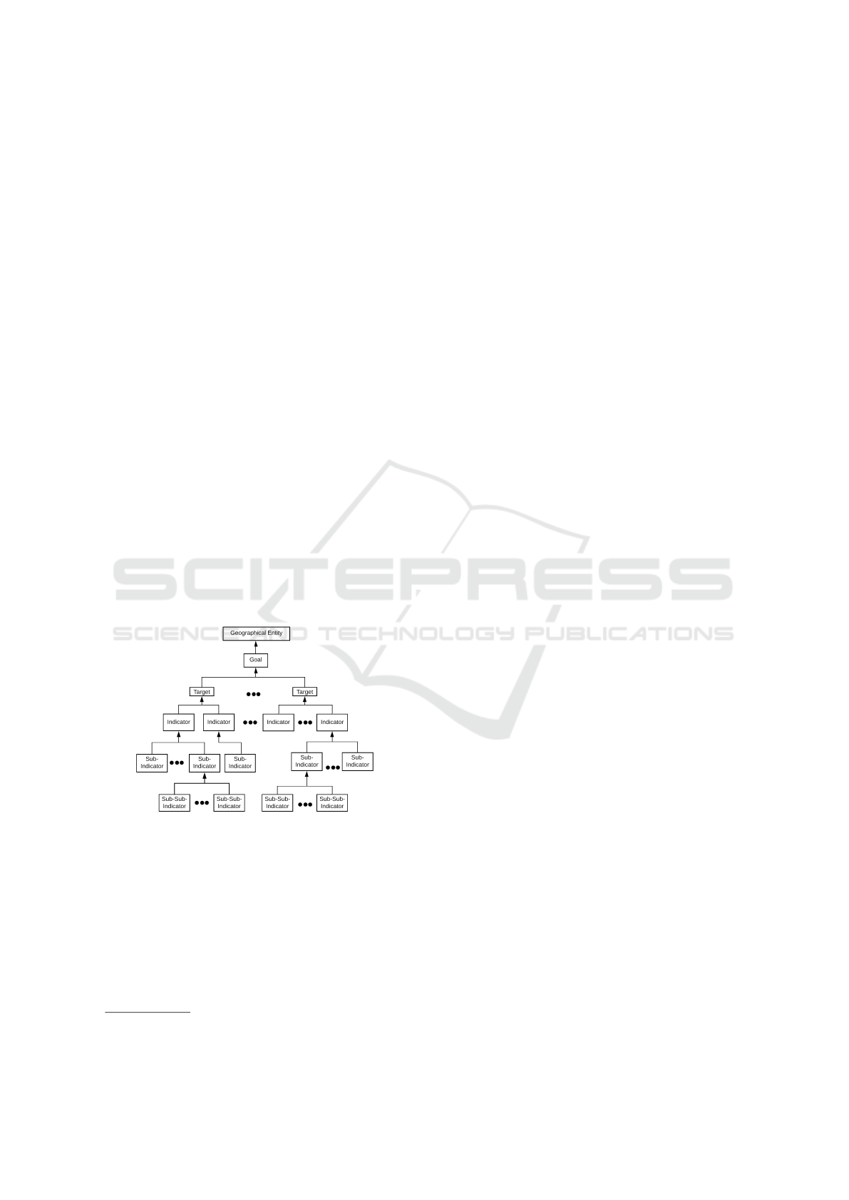
Figure 1: The hierarchical nature (taxonomy) of SDG data.

The nature of the SDG data associated with an in-

dividual geographic entity can be conceptualised in

the form of a hierarchy as shown in Figure 1 as ﬁrst

proposed in (Alharbi et al., 2019), and later adopted in

(Alharbi et al., 2020). The hierarchy describes both a

taxonomy for the SDG data and an operational frame-

work. Inspection of the ﬁgure indicates that each goal

comprises a set of targets, which in turn are depen-

dent on a set of indicators, sub-indicators, and even

https://unstats.un.org/SDGs/indicators/database/

sub-sub-indicators. Sub-sub indicators contribute to

sub-indicators, sub-indicators to indicators and so on

to the root of the tree. Not every indicator is rele-

vant to every geographic entity, for example foresta-

tion has little applicability in Saudi Arabia.

Unlike other hierarchical data formats, such as

ﬁnancial indexes or tourism data (Athanasopoulos

et al., 2009), where data exists in multiple levels and

is interpreted in a top-down manner, the SDG hier-

archy in Figure 1 is interpreted in a bottom-up man-

ner . Starting from the leaf nodes, a boolean value is

generated and passed up the tree. At the leaf nodes

this is generated using a function f (v) where v is a

value generated using a prediction model which is

compared to a threshold σ as shown in Equation 4.

For the intermediate nodes the boolean values are

generated using a simple “logical and” operation ac-

cording to the input from the immediate child nodes.

The predictor used in (Alharbi et al., 2019) were uni-

variate time series predictors (FBProphet was advo-

cated), those used in (Alharbi et al., 2020) were multi-

variate LSTMs, the number of dimensions depended

on the number of causality relationships that were

identiﬁed with respect to each leaf node, if no rela-

tionships were found with respect to a given indicator

the multi-variate prediction reduced to a uni-variate

prediction. A broadly similar approach is proposed

with respect to the SDG-TTF methodology presented

in this paper.

f (v) =

(

true if v > σ

false otherwise

(4)

The data held at the leaf nodes of the tree given in

Figure 1, regardless of whether these nodes represent

indicators, sub-indicators or sub-sub-indicators, is in

the form of a series of time stamped values; in other

words each leaf node holds a time series. The max-

imum number of points, as of October 2019, in any

one time series is 20. However, there are many miss-

ing values, especially for 2018 and 2019 which means

that, in effect, there are no more that 18 values typi-

cally available. Figure 2 shows the number of miss-

ing values per year for the geographic region “North

Africa” (the year 2019 has been omitted). From the

ﬁgure it can be observed that there are large num-

bers of missing values for 2017 and 2018. The rea-

son for missing values varies, from Missing Com-

pletely at Random (MCAR) to Missing Not at Ran-

dom, (MNAR) (Heitjan and Basu, 1996). An exam-

ple of the ﬁrst can be found for the geographic re-

gion “Egypt” and Indicator 1.2.1 (Goal 1, Target 2,

Indicator 1), “Proportion of population living below

the national poverty line(per cent)”, where only data

for the random years 2003, 2007 2009 is available.

DeLTA 2021 - 2nd International Conference on Deep Learning Theory and Applications

126

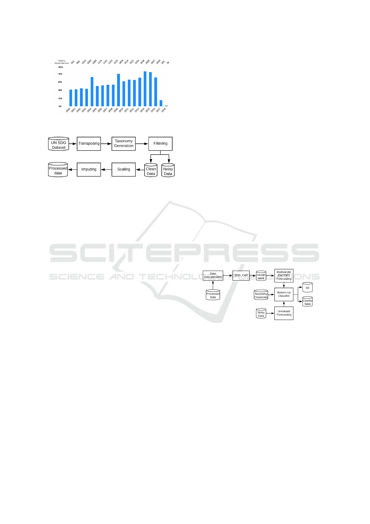
Figure 2: Missing values in UN North Africa region per

year from 2000 to 2018.

Figure 3: An overview of the SDG-TTF data pre-processing

workﬂow.

An example of the second, again for geographic re-

gion “Egypt”, can be found for the Indicator 15.2.1,

“By 2020, promote the implementation of sustainable

management of all types of forests, halt deforestation,

restore degraded forests and substantially increase af-

forestation and reforestation globally” where data is

collected on a ﬁve year cycle; in other words there are

regular 5 year gaps between recorded data items.

In addition to the length of the time series, fur-

ther challenges include: (i) the wide verity of different

scales and data types used in the time series, (ii) the

variability in the nature of the time series and (iii) the

nature of the σ threshold at the individual leaf nodes.

The ﬁrst can best be illustrated by an example. If we

consider Indicators 1.5.2, “Direct agricultural loss at-

tributed to disaster (millions of current United States

dollars)”, and Indicators 7.1.1, “Proportion of popu-

lation with access to electricity, by urban/rural (per-

centage)”, the ﬁrst is reported in millions of US dol-

lars whilst the second is reported as a percentage. The

second challenge can be illustrated by observing that

some time series remain at zero with only occasional

peeks, for example in the case Indicator 1.5.2 (“disas-

ters” do not happen every year); whilst other time se-

ries increase steadily year on year, for example with

respect to Indicator 7.1.1 ”proportion of population

with access to electricity”. The threshold issue re-

quires particular consideration, not all SDG indicators

specify a threshold, as can be seen by contrasting In-

dicators 1.5.2 and 7.1.1; Indicator 1.5.2 does not ref-

erence a threshold. The solution is beyond the scope

of this paper, hence the thresholds used in (Alharbi

et al., 2019) were adopted.

4 SDG DATA PREPROCESSING

Given the foregoing the SDG data requires consider-

able preprocessing. Figure 3 presents an overview of

the preprocessing required prior to the application of

the proposed SDG-TTF system. It should be noted

here that this preprocessing only needs to be done

once, or at last only once for each update of the SDG

data. From the ﬁgure the preprocsessing is conducted

in ﬁve steps: (i) transposing, (ii) taxonomy genera-

tion, (iii) ﬁltering, (iv) scaling, (v) Imputing. The

preprocessing commences with the transposing of the

raw 19 × 38 row-column format (for each leaf node)

to a 1 × 24 row-column format (for each leaf node):

hGR, G, T, , D,t

, . . . ,t

i (5)

The data is then ﬁltered based on the number miss-

ing values. Any time series with more than 15 missing

values or featuring irregularities such as the presence

of ﬁve zeros in a row, is deemed to be noisy data and is

put to one side in a set T

noise

= {T

, T

, . . . }. The rest

of the data will then be scaled using RobustScaler (Pe-

dregosa, 2011), and then any missing values will be

imputed using Spline (Pedregosa, 2011). In practice,

as illustrated in Figure 2, we have found it appropri-

ate to use data from 2000 to 2017 inclusive because

of the large number of missing values for 2018 and

2019. The ﬁnal output is a set T = {T

, T

, . . . }.

Figure 4: Overview of the SDG-TTF workﬂow.

5 THE SDG TRACK, TRACE AND

FORECAST (SDG-TTF) MODEL

This section presents the proposed SDG-TTF frame-

work. The workﬂow for the framework is presented

in Figure 4. The input is the set of time series, T =

, T

, . . . }, from the previous pre-processing stage

as described above. From the ﬁgure it can be seen that

the SDG-TTF framework comprises ﬁve processes:

(i) Data Grouping (ii) Relation Discovery, (iii) mul-

tivariate ENC/DEC Forecasting, (iv) univariate fore-

casting and (v) bottom-up classiﬁcation. Note that

two forecasting processes, Multivariate ENC/DEC

and univariate, feed into the bottom up classiﬁcation.

Sustainable Development Goals Monitoring and Forecasting using Time Series Analysis

127

During the data grouping process T is grouped

into geographic regions. Recall that the objective of

this paper is to improve on current SDG prediction

effectiveness by taking into consideration causalities

between countries and their neighbours, something

not considered in previous work. The data group-

ing was conducted using geographic area codes based

on the UN regional segmentation

. For example, the

seven countries Algeria, Egypt, Libya, Morocco, Su-

dan, Tunisia and Western Sahara were grouped into

the UN sub region of North Africa. Any other group-

ing mechanism would be equally applicable.

The next process is to determine the relationship

between the time series in T. Each T

∈ T is compared

to its complement T

= {x ∈ T : x 6= T

}). The in-

teraction between each time series is measured using

a causality ranking measure r. This is calculated, us-

ing RMSE, as described in Sub-section 2.2. For the

evaluation presented in this paper the six time series

causality mechanisms listed in Section 2 were used

(Lasso, R

, Pearson Correlation, Mann-Whitney

U Test, Granger and ACA). For each T

, the time se-

ries in T

were then ranked according to r and the top

k selected for further processing, the set of time series

. For the evaluation presented later in this paper

k = 50 was used. Each T

and T

was then stored

in a “causer table”, T

causer

= {τ

, τ

, . . . }, where τ

∪ T

For each τ

∈ T

causer

the next process in the work-

ﬂow shown Figure 4 was to build a multi-variate time

series forecasting model. A range of tools and tech-

niques are available whereby such a model can be

constructed. However, for the evaluation presented

later in this paper a multi-variate LSTM-Encoder-

Decoder (Enc-Dec) (Jason, 2018) was used. Recall,

from the previous section, that during data prepro-

cessing time series which were deemed unusable with

respect to the determination of causality relationships

were set aside in a noise set T

noise

= {T

, T

, . . . }.

However, although unsuited to causality relationship

determination this data can still be used for the pur-

pose of forecasting SDG attainment. For each time

series T

∈ T

noise

a uni-variate time series forecasting

model was built. Again there are a number of tools

and techniques available whereby such a model can

be constructed. For the evaluation presented in the

following section uni-variate FBPprophet was used.

The ﬁnal process in the SDG-TTF workﬂow is the

classiﬁcation process where we ascertain whether a

given country will meet its SDG goals or not using

the generated multi-variate and uni-variate time se-

ries forecasting models described above. The funda-

https://unstats.un.org/sdgs/report/2019/regional-groups/

mental process is similar to that presented in (Alharbi

et al., 2019) where an alternative SDG attainment

prediction framework was presented (the SDG-CAP

framework), which in turn was founded on the same

hierarchical topology described in (Alharbi et al.,

2020) and described in Section 3. The results are

stored in a “country table” and can be visualised using

D3.js (Bostock et al., 2011). An example of the latter

is given and discussed in Section 7 (Figure 5).

6 EVALUATION

The evaluation of the proposed SDG-TTF model is

presented in this section. For the evaluation the UN

North Africa sub-region was considered. This com-

prised a total of 3667 time series (leaf nodes in the

topology), covering the 17 SDGs with respect to the

North Africa sub-region of which 2325 were placed in

T and the remainder in T

noise

. The substantial number

of time series allocated to T

noise

was due to the large

number of missing values that featured in the North

Africa sub region SDG data (see Figure 2). The ob-

jectives of the evaluation were:

1. To determine the most appropriate causality dis-

covery mechanism for use with SDG-TFF

2. To determine whether by taking into considera-

tion both intra-region and inter-region causality

relationships better SDG predictions could be pro-

duced.

For the evaluation the input data was divided into

14 observations for training and 4 observations for

testing; k = 50 was used through out. All experiments

were run on a windows 10 machine running under

Ryzen 9 CPU, RTX 2060 GPU, 16 GB of RAM and

1TB SSD. Comparisons were made with the SDG-

AP and SDG-CAP prediction frameworks presented

in (Alharbi et al., 2019) and (Alharbi et al., 2020)

respectively. All algorithms were implemented us-

ing the Python programming language. The evalua-

tion metric used was RMSE (Root Mean Squared Er-

ror). As noted earlier, six different causality discov-

ery mechanisms were considered: Lasso, R

, Pear-

son Correlation, Mann-Whitney U Test, Granger and

ACA. Detail of the results obtained are given in Ta-

ble 1 and 2 for Algeria and 12 selected SDGs. The

Table gives the RMSE error for each SDG when the

last four points are predicted with respect to each time

series; best results are highlighted in bold font. The

overall average RMSE value is given at the bottom

of the table, for each approach considered, together

with the associated standard deviation. The ﬁrst two

columns in the table give the sequential time series ID

DeLTA 2021 - 2nd International Conference on Deep Learning Theory and Applications

128

Table 1: A sample of RMSE values for selected SDG indicators for Algeria.

Time Series Code SDG-TTF SDG-CAP SDG-AP

Lasso R

Pearson

correlation

T test

Granger

Causality

ACA ACA

Univariate

LSTM

FBProphet

1 SH DTH RNCOM M DIA 0.089 0.096 0.150 0.133 0.079 0.106 0.252 34.039 NaN

2 SH DYN NMRTN MF 0.166 0.166 0.143 0.109 0.151 0.169 0.102 290.937 5.346

3 SH DTH NCOM F 0.056 0.665 0.044 0.027 0.045 0.093 0.072 0.196 NaN

4 SH DTH NCOM M 0.032 0.048 0.062 0.077 0.080 0.050 0.058 0.398 NaN

5 SH STA POISN F 0.095 0.110 0.097 0.099 0.170 0.082 0.152 0.010 0.009

6 SH STA POISN M 0.337 0.237 0.325 0.391 0.296 0.235 0.141 0.041 0.038

7 DC TOF HLTHL 0.196 0.107 0.103 0.107 0.105 0.094 0.283 10.664 NaN

8 SH STA SCIDEN F 0.094 0.088 0.118 0.080 0.079 0.066 0.117 6.599 NaN

9 SH STA SCIDEN M 0.067 0.894 0.416 0.190 0.086 0.087 0.071 0.094 0.044

10 SH STA SCIDE MF 0.057 0.110 0.079 0.052 0.070 0.109 0.218 0.098 0.035

11 SH STA SCIDE F 0.070 0.102 0.103 0.091 0.084 0.135 0.580 0.078 NaN

12 SH DYN MORTN MF 0.283 0.268 0.295 0.185 0.250 0.257 0.110 355.882 217.944

Average 0.129 0.241 0.161 0.128 0.125 0.124 0.180 58.253 37.236

Standard Deviation 0.093 0.253 0.113 0.091 0.075 0.062 0.139 119.684 80.838

number (to support ease of reading) and the unique

descriptor, which, as noted earlier, allows it to be re-

lated back to a speciﬁc SDG indicator, sub-indcator

or sub-sub-indicator. The following six columns give

the RMSE values using SDG-TTF combined with the

six causality mechanisms considered. It can be seen

that ACA, the hybrid causal relationship discovery

approach suggested in (Alharbi et al., 2020), pro-

duced the best overall result. The seventh column

in the table gives the RMSE value using the SDG-

CAP SDG attainment prediction framework proposed

in (Alharbi et al., 2020), coupled with ACA to give

best results. Recall that using SDG-CAP only intra-

entity (single country) causal relationships were con-

sidered, as opposed inter-entity causal relationships

as in the case of SDG-TTF. From the table it can be

seen from the recorded average RMSE results that the

proposed SDG-TTF framework out-performed SDG-

CAP. The ﬁnal two columns give the result with re-

spect to SDG-AP (Alharbi et al., 2019). Recall that

SDG-AP does not feature any consideration of the

possibility of causality relationships. Predictions are

made using a single time series, uni-variate, approach.

For SDG-AP two prediction models were considered

LSTM and FBProphet. From Table 1 it can be seen,

from the recorded average RMSE results, that SDG-

TTF out-performed SDG-AP and SDG-CAP. Table

2 represent a summary of the results obtained from

the entire North Aftica. Overall it can be concluded

that consideration of inter-entity causal relationships,

as well as intra-entity causal relationships, as incor-

porated into the SDG-TTF framework results in im-

proved SDG attainment prediction; and that the most

appropriate causality discovery mechanism was the

ACA mechanism.

Table 2: Total Averages for North Africa per country.

Country

SDG-TTF

(ACA)

SDG-CAP

(ACA)

SDG-AP

(FBProphet)

RMSE AVG SD AVG SD AVG SD

Algeria 0.3 0.5 0.4 0.9 0.8 7.6

Egypt 0.4 1.4 0.5 2.0 0.6 3.1

Libya 0.8 1.1 0.9 1.0 0.6 0.8

Morocco 0.6 0.3 0.5 1.4 0.6 1.3

Sudan 0.2 0.2 0.3 0.3 0.4 0.4

Tunisia 0.4 0.8 0.5 1.1 0.7 1.8

Western

Sahara

0.5 0.3 0.6 0.5 0.8 0.5

Average 0.4 0.7 0.5 1.0 0.6 2.2

7 SYSTEM OPERATION

The operation of the proposed SDG-TTF framework

was investigated using a number of case studies. One

such case study is presented here. Namely, SDG

3, Target 2 (Target 3.2): “By 2030, end preventable

deaths of newborns and children under ﬁve years of

age, with all countries aiming to reduce neonatal mor-

tality to at least as low as 12 per 1000 live births and

under-5 mortality to at least as low as 25 per 1000 live

births”, and the country Algeria. Target 3.2 comprises

two indicators (3.2.1 and 3.2.2), each comprised of 4

and 1 sub-indicators respectively. Note that there are

two threshold here, ≤ 12 for live births (interpreted as

aged less than 1 month old) and ≤ 25 for under ﬁve

years old.

SDG-TTF was then used to make predictions up

to the year 2030. The generated output is a “country

table”, as indicated in the workﬂow presented in Fig-

ure 4. A fragment of this table for Target 3.2 is given

in Table 3.

The ﬁrst four columns give details of each sub-

sub-indicator. The ﬁfth column gives the threshold for

Sustainable Development Goals Monitoring and Forecasting using Time Series Analysis

129

Table 3: Forecast results for Target 3.2, the year 2030 and

the country Algeria.

Indicator Age/Sex Initial Target Forecast Result

3.2.1 1Y/F 20.2 <=25 16.94 Met

3.2.1 1Y/M 22.9 <=25 20.82 Met

3.2.1 5Y/F 23.7 <=25 19.89 Met

3.2.1 5Y/F 26.6 <=25 24.13 Met

3.2.2 1Month/FM 15 <=12 13.75 Not Met

Figure 5: Vitalising SDG attainment using D3.js.

each indicator The sixth and seventh columns, “Initial

Value” and “Prediction”, gives the mortality value per

1000 live births in 2015, and the predicted value in

2030. The ﬁnal SDG attainment prediction result is

given in the last column. For Target 3.2 to be attained

(met), the value associated with each indicator (time

series) must meet its threshold (at or below the rele-

vant threshold in this case). Unfortunately, in this ex-

ample, all of the indicators meet the required thresh-

old before 2030 except 3.2.2. Thus it is concluded

that Target 3.2 will not be attained.

The SDG-TTF framework includes a visualisation

mechanism, as indicated in Figure 4. This was imple-

mented using D3.js (Bostock et al., 2011). The vi-

sualisation allows users to: (i) track the progress of

different goals over a given time frame, and (ii) trace

the achievement of individual bottom level indicators

in an interactive manner. An example of such visual-

isations is given in Figure 5 using the case study pre-

sented above. From the ﬁgure it can be seen that using

the visualisation it is easy to identify goal attainment

(or non-attainment as in this case). Nodes coloured

in green highlight indicators/targets/goals that will be

attained on time. Nodes coloured in red highlight in-

dicators/targets/goals that will not be attained on time.

For a more detailed analysis of why a goal is not at-

taining the relevant country table can give a better ex-

planation.

8 CONCLUSION

In this paper we have presented the SDG-TTF attain-

ment prediction framework. Unlike previous frame-

works directed at SDG attainment prediction the

SDG-TTF framework takes into consideration both

inter- and intra-geographic entity (county, region)

causal correlation. The intuition was that individ-

ual SDG indicators should not be considered in isola-

tion because inspection of the indicators demonstrates

clear potential for causal relationships with respect to

other indicators for the entity in question and with re-

spect to indicators in neighbouring entities. The eval-

uation of the framework demonstrates that more ro-

bust SDG attainment predictions using SDF-TTF can

be made. For future work the authors intend to inves-

tigate further alternative causal relationship discovery

mechanisms; and to give further consideration of the

parameter k, the number of time series to be included

when building the multi-variate time series prediction

models central to the SDG-TTF framework. Finally

the authors intend to use the framework to investigate

the effect on SDG attainment in presence of natural

disasters, such as the Covid-19 pandemic, which oc-

cur for short periods of time but might have a signiﬁ-

cant impact on SDG attainment prediction.

REFERENCES

Alam, N. and Rudin, C. (2015). Robust Nonparametric

Testing for Causal Inference in Observational Studies.

Optimization Online, Dec, pages 1–39.

Alharbi, Y., Arribas-Bel, D., and Coenen, F. (2019).

Sustainable development goal attainment prediction:

A Hierarchical Framework using Time Series Mod-

elling. IC3K 2019, 1:297–304.

Alharbi, Y., Coenen, F., and Arribas-Bel, D. (2020). Sus-

tainable development goal relational modelling: In-

troducing the SDG-CAP methodology. In DAWAK),

volume 12393 LNCS, pages 183–196.

Athanasopoulos, G., Ahmed, R. A., and Hyndman, R. J.

(2009). Hierarchical forecasts for Australian domestic

tourism. IFJ, 25(1):146–166.

Bostock, M., Ogievetsky, V., and Heer, J. (2011). D3 data-

driven documents. IEEE TVCG, 17.

Chen, K., Zhou, Y., and Dai, F. (2015). A LSTM-based

method for stock returns prediction: A case study of

China stock market. In IEEE Big Data 2015. IEEE.

De Gooijer, J. G. and Hyndman, R. J. (2006). 25 Years of

Time Series Forecasting. IFJ, 22(3):443–473.

Deschamps, E. (2004). The impact of institutional change

on forecast accuracy: A case study of budget forecast-

ing in Washington State. IFJ, 20(4):647–657.

orgo, G., Sebesty

en, V., and Abonyi, J. (2018). Evaluating

the interconnectedness of the sustainable development

goals based on the causality analysis of sustainability

indicators. Sustainability (Switzerland), 10(10):3766.

Epprecht, C., Guegan, D., and Veiga,

A. (2013). Com-

paring variable selection techniques for linear regres-

sion: LASSO and Autometrics. Centre d’

economie de

la Sorbonne.

Frey, B. B. (2018). Pearson Correlation Coefﬁcient. In The

SAGE Encyclopedia of Educational Research, Mea-

surement, and Evaluation, pages 1–4. Springer.

DeLTA 2021 - 2nd International Conference on Deep Learning Theory and Applications

130

Heitjan, D. F. and Basu, S. (1996). Distinguishing “missing

at random” and “missing completely at random”. The

American Statistician, 50(3):207–213.

Hyndman, R. and Kostenko, A. (2007). Minimum sam-

ple size requirements for seasonal forecasting models.

Foresight, 6(Spring):12–15.

Jason, B. (2018). Deep Learning For Time Series Forecast-

ing, volume 1. Machine Learning Mastery.

Narayan, P. K. and Smyth, R. (2009). Multivariate granger

causality between electricity consumption, exports

and GDP: Evidence from a panel of Middle Eastern

countries. Energy Policy, 37(1):229–236.

Nauta, M., Bucur, D., and Seifert, C. Causal discovery with

attention-based convolutional neural networks. Ma-

chine Learning and Knowledge Extraction, 1(1).

Pedregosa (2011). Scikit-learn: Machine learning in

python. Journal of Machine Learning Research, 12.

Qing, X. and Niu, Y. Hourly day-ahead solar irradiance

prediction using weather forecasts by LSTM. Energy.

R Gonz

alez, L., B, D., M, L. F., and V, R. (2019). Long-

term electricity supply and demand forecast (2018-

2040): A LEAP model application towards a sustain-

able power generation system in Ecuador. Sustain-

ability (Switzerland), 11(19):5316.

Seabold, S. and Perktold, J. (2010). Statsmodels: Econo-

metric and Statistical Modeling with Python. In the

9th Python in Science Conference, pages 92–96.

T, A., L, N., S, G., Ps, D., and K, M. (2020). Efﬁciency

forecasting for municipal solid waste recycling in the

context on sustainable development of economy. In

E3S Web of Conferences, volume 166, page 13021.

Tibshirani, R. (1996). Regression Shrinkage and Selection

Via the Lasso. JRSS.

UN, S. D. (2559). E-Handbook on Sustainable Develop-

ment Goals Indicators.

United Nations (2015). The Millennium Development

Goals Report. United Nations, page 72.

Sustainable Development Goals Monitoring and Forecasting using Time Series Analysis

131