Genetic Optimization of Excitation Signals for Nonlinear Dynamic

System Identiﬁcation

Volker Smits

1 a

and Oliver Nelles

2 b

DEUTZ AG, Ottostr. 1, Cologne, Germany

Department of Mechanics and Control - Mechatronics, University of Siegen, Paul-Bonatz-Str. 9-11, Siegen, Germany

Keywords:

Design of Experiment, Genetic Algorithm, System Identiﬁcation of Nonlinear Dynamic Systems, Optimal

Excitation Signals, APRBS, GOATS.

Abstract:

Two new methods for optimization of passive step-based excitation signals for system identiﬁcation of non-

linear dynamic processes via a genetic algorithm are introduced - an optimized Amplitude Pseudo Random

Binary Signal (APRBS

Opt

) and a Genetic Optimized Time Amplitude Signal (GOATS). The investigated op-

timization objectives are the evenly excitation of all frequencies and the uniform data distribution of the space

spanned by the system’s input and output. The results show that the GOATS optimized according to the

uniform data distribution outperform the state-of-the-art excitation signals standard ARPBS (APRBS

Std

), Op-

timized Nonlinear Input Signal (OMNIPUS), Chirp and Multi-Sine in the achieved model quality on three

artiﬁcially created Single-Input Single-Output (SISO) nonlinear dynamic processes. However, the APRBS

Opt

only exceeds the Chirp, Multi-Sine and APRBS

Std

in the achievable model quality. Additionally, the GOATS

can be used for stiff systems, supplementing existing data and easy incorporation of constraints.

1 INTRODUCTION

System identiﬁcation refers to a process of build-

ing mathematical models of a dynamic or static sys-

tem based on the relation between measured input-

output data of a given system (Isermann, 1992; Hart-

mann, 2013). The quality of such data-based mod-

els is mainly inﬂuenced by the information which

are gathered in the data for the model training (train-

ing data) (Hartmann, 2013; Heinz and Nelles, 2017;

Heinz et al., 2017; Tietze, 2015). A well-known and

validated methodology for the maximization of the

amount of information of the training data is the De-

sign of Experiment (DoE) (Hartmann, 2013). The

DoE for the training of dynamic models (dynamic

DoE) differs from the DoE for training of stationary

models (static DoE) regarding the kind of information

needed to be collected during the experiment. Both

the dynamic and the stationary models need the in-

formation about the stationary nonlinearity (equilib-

rium), whereas the dynamic model needs additional

information about the frequency and the transient be-

haviour of the systems.

https://orcid.org/0000-0001-8004-7957

https://orcid.org/0000-0002-9471-8106

In general, two classes of DoE can be distinguished:

The passive and the active DoE. The passive DoE, de-

ﬁnes the ofﬂine development of an experiment design,

whereas the active DoE describes the online approach

of a DoE (Heinz and Nelles, 2017). We assume that

the optimization task of dynamic DoE’s of complex

nonlinear dynamic systems is too difﬁcult to solve

properly online in the limited time range. To address

this problem, simpliﬁcations of the optimization task

often have to be chosen such as simpler model struc-

tures or less computational demanding loss functions.

This, however, results in only optimal solutions for

the chosen simpliﬁcations. For this reason, the cur-

rent paper aims to develop two new passive excitation

signals to increase the modeling quality of nonlinear

dynamic processes.

Chirp, Multi-Sine and Amplitude Pseudo Random

Binary Signal (APRBS) are widely used passively

designed excitation signals (Baumann et al., 2008;

Hoagg et al., 2006; Nelles, 2013; Pintelon and

Schoukens, 2012; Rivera et al., 2002; Tietze, 2015).

Step-based excitation signals like an APRBS show a

better capability to cover the space spanned by the

system’s input u and output y compared to sinusoid-

based signals such as Chirp and Multi-Sine (Heinz

138

Smits, V. and Nelles, O.

Genetic Optimization of Excitation Signals for Nonlinear Dynamic System Identiﬁcation.

DOI: 10.5220/0010545501380145

In Proceedings of the 18th International Conference on Informatics in Control, Automation and Robotics (ICINCO 2021), pages 138-145

ISBN: 978-989-758-522-7

and Nelles, 2017). In the last decade, a variety of opti-

mizations and modiﬁcations of the APRBS have been

developed (Deﬂorian and Zaglauer, 2011; Heinz and

Nelles, 2016; Nouri et al., 2018).

To the best of our knowledge, the study of Nouri et

al. is the ﬁrst study which optimized an APRBS via

a genetic algorithm (GA) (Nouri et al., 2018). They

have optimized the APRBS according to an informa-

tion criterion to minimize the uncertainty for a pa-

rameter estimation of a predeﬁned white box model

structure. In their study, the optimization is used to

improve the parameter identiﬁcation instead of sys-

tem identiﬁcation. Another modern step-based signal

is the Optimized Nonlinear Input Signal (OMNIPUS),

which is proposed in (Heinz and Nelles, 2017; Heinz

et al., 2017). It aims to optimize the coverage of the

space spanned by u and y. However, the optimiza-

tion of OMNIPUS is incrementally, which can lead

to suboptimal designs, because earlier designed se-

quences of the optimization cannot be changed in the

later process of the optimization.

The present paper aims to add to the current literature

by developing two new passive excitation signals for

system identiﬁcation of nonlinear dynamic systems

which will be compared to four state of the art ex-

citation signals on three artiﬁcially created processes.

Our approach differs from the current studies regard-

ing the optimization of a step-based excitation signals

by introducing new loss functions for optimizing the

coverage of the space spanned by u and y and the

evenly excitation of all frequencies in a global fash-

ion via a GA.

2 METHOD

2.1 Design of Experiment

The ﬁrst investigated optimization objective is the

evenly excitation of all frequencies f

which aims

to the excitation of the relevant bandwidth of sys-

tem without over-emphasizing speciﬁc frequencies.

The second investigated optimization objective is the

space-ﬁlling coverage f

of the space spanned by the

system’s input u and output y or more precisely the

input space of a Nonlinear AutoRegressive with eX-

ogenous input (NARX) system. Since the regressors

of the regression matrix X e.g. of a ﬁrst order NARX

structure are the delayed sequences of input u(k − 1)

and output y(k − 1), the optimization of the space

spanned by these regressors seems to be purposeful

to improve the modeling quality.

In Fig. 1 the ﬁrst order NARX input space of a non-

linear dynamic process separately excited with a stan-

0.5

u(k − 1)

y(k − 1)

APRBS

Std

0.5

u(k − 1)

Chirp

0.5

u(k − 1)

Multi-Sine

Figure 1: First order NARX input space point distribution

of an APRBS, a Chirp and Multi-Sine.

dard APRBS

Std

, Chirp and Multi-Sine is shown. As

Heinz and Nelles have shown and also is illustrated

in Fig. 1 step-based signals have a better space cov-

erage compared to sinusoidal-based signals in the

ﬁrst order NARX input space (Heinz and Nelles,

2017). Sinusoidal-based signals like the Multi-Sine

and Chirp signal are not able to ﬁll the areas in the

upper left and lower right corner. Step-based signals

like the APRBS and OMNIPUS are able to cover the

upper left and lower right corner as well as the center

due to their piecewise constant sequences and their

steps (Heinz and Nelles, 2017). Due to this reason,

the signal type of step-based signals is considered for

the two new excitation signals which are optimized

via a GA.

The ﬁrst new signal type is an optimized

APRBS (APRBS

Opt

) with an optimized amplitude

permutation p

. An APRBS is based on a se-

quence which controls the duration of the con-

stant phases and the time dependent occurrence of

the steps. This sequence is generated by a pseu-

dorandom binary sequence (PRBS). The minimum

hold time T

allows to adjust the APRBS to a

speciﬁc frequency range (Isermann, 1992; Nelles

and Isermann, 1995). The different amplitude levels

A = N

× d (N

:= amount of amplitude levels, d :=

input dimension) could be chosen prior e.g. by a static

DoE method and then modulated to the PRBS sequen-

tially (Isermann, 2010). The permutation of these

amplitudes p

will deﬁne the amplitude order of the

APRBS

Opt

which inﬂuences the coverage of the in-

put space and the amplitude spectrum, whereby it is a

promising parameter for the optimization. The second

new signal type is inspired by the APRBS as well. For

this signal type not only the amplitude order p

is op-

timized via a GA, but also the sequence p

. Therefore,

it is an independent new signal type and is named Ge-

netic Optimized Amplitude Time Signal (GOATS).

2.2 Genetic Algorithm

A GA is a metaheuristic algorithm which belongs to

the family of evolutionary algorithms (EA). The basic

concept is to imitate the Darwinian principle of evo-

Genetic Optimization of Excitation Signals for Nonlinear Dynamic System Identiﬁcation

139

lution (variation, reproduction and selection) to tech-

nical environment to iteratively solve optimization

problems (Holland, 1975; Sivanandam S.N., 2008).

Therefore, a GA is suitable to optimize the introduced

parameters of the last subsection the permutation p

and the sequence p

without information about the

derivatives.

The used GAs for single objective optimization

(SOO) and multi objective optimization (MOO) of

the objectives f

and f

in this paper are a combi-

nation of different methods for selection, recombina-

tion and mutation of popular genetic algorithms due

to their good performance. The Tournament Selec-

tion is commonly used and very popular method for

selection due to its efﬁciency and simple implementa-

tion (Goldberg and Deb, 1991; Razali and Geraghty,

2011). In this paper, it is used in selection of recom-

bination candidates and the candidates for the next

generation. In the SOO, the ﬁtness of the individu-

als is directly compared with a set of four individuals.

The MOO uses the tournament selection of the Non-

dominated Sorting Genetic Algorithm II (NSGA-II)

proposed in (Deb et al., 2000).

The two parameter types of the optimization are the

permutation p

∈ N

of the APRBS and GOATS and

the sequence p

∈ N

of the GOATS. The permuta-

tion p

deﬁnes the order of the different amplitude

levels of the ARPBS and the GOATS. The sequence

is represented as a sequence of integers between

two limits which are deﬁning the minimum and max-

imum duration of an amplitude level of the GOATS.

As crossover operator of the permutation parameter

the Order Crossover 1, Order Crossover 2, Partially

Map Crossover and Position Based Crossover are

used (Davis, 1985; Goldberg et al., 1985; Syswerda,

1991). Which speciﬁc crossover method in a

crossover situation is chosen, is depending on a uni-

form random distribution. This concept of a uni-

form selection is analogous implemented for the the

mutation operators, whereby every method can con-

tribute with its advantages. The mutation operators of

the permutation are the Reverse-, Interchanging- and

One-Point-Slide-Mutation

(Sivanandam S.N., 2008).

The mutation operator used for the sequence param-

eter type is the Power-Mutation (Deep et al., 2009).

It is used to produce new genes for the sequence.

As crossover operators of the sequence parameter

type the Uniform-, SBX- and Two-Point-Crossover

are taken (Deb and Agrawal, 1995; Hartmann, 1998).

The SBX-crossover is slightly adapted by a round-

Slides a subtour for one position, Example: Parent: [7,

10, 5, 3, 4, 2, 8, 9, 6, 1]; Subtour: [3, 4, 2]; Child:[7, 10, 3,

4, 2, 5, 8, 9, 6, 1]

function, so that after the crossover the sequence only

contains integers.

Additionally, the mutation rate λ

and crossover rate

are adaptively changed during optimization by rat-

ing the normalized relative improvement of the ﬁtness

caused by the mutation or crossover. This approach is

inspired by the work of Lin et al. (Lin et al., 2003).

2.3 Modeling Approach for Nonlinear

System Identiﬁcation

Besides a good space-ﬁlling of the training data and

good coverage of frequency spectra, the question

arises how the quality of an excitation signal can

be quantiﬁed. A straightforward and reasonable ap-

proach is to quantify the quality of an excitation signal

for nonlinear system identiﬁcation whilst a model is

trained based on the data which is gathered by the ex-

citation signal. While it is too computational expen-

sive and impractical to use this directly in a GA, for

rating the results of the optimization it is well suited.

A deterministic model training is preferable, because

a nondeterministic training would impede the analysis

due to a more complicated distinction of the reasons

of the change of the model performance. One model

architecture which is easy to train by the usage of a

deterministic training method and yields good model

performances, is the architecture of local model net-

works (LMN) (Hartmann, 2013; Nelles, 2013). For

the optimization of the LMN the hierarchical local

model tree (HILOMOT) is used (Nelles, 2006). The

HILOMOT is an incremental tree construction algo-

rithm which divides the input space in an axis-oblique

manner and estimates local models in the created sub-

spaces. The overall model output ˆy is calculated by

the weighted sum of the sub-models ˆy

(x) and the val-

idation functions Φ

(z) with the subsets x and z of all

inputs u (Nelles, 2006).

ˆy(x,z) =

∑

i=1

ˆy

(x) · Φ

(z) , where

∑

i=1

(z) = 1 (1)

3 LOSS FUNCTIONS AND

OPTIMIZATION PROBLEMS

For rating the space-ﬁlling property of a point dis-

tribution, loss functions are required to quantify the

coverage of the points in a space-ﬁlling sense. For

the quantiﬁcation of the coverage of the input space

three different loss function are investigated. The con-

sidered input space in this survey is the NARX input

space X. For the later usage and simplicity they will

ICINCO 2021 - 18th International Conference on Informatics in Control, Automation and Robotics

140

be gathered under the term input space-loss functions

• Audze Eglais (AE) (Audze and Eglais, 1977)

∑

i=1

∑

j=i+1

i j

, where L

i j



− X



(2)

• Maximum Projection (MP) (Joseph et al., 2015)

(





N−1

∑

i=1

∑

j=i+1

∏

l=1

− x

)

1/p

(3)

• Fast and Simple Dataset Optimization (FA) (Peter

and Nelles, 2019)

∑

i=1

|1 − ˆq(X(i))|, (4)

where ˆq(X(i)) =

∑

i=1

−

[X−X(i)]

−1

[X−X(i)]

(2π)

|Σ|

Σ = diag(σ

,σ

,. .. ,σ

)

The AE and MP belong to the maximin distance de-

signs which mainly penalize close points in the input

space. The MP is based on the AE criterion and tries

to extend its projection properties in the subspaces of

the given input space but is computational more ex-

pensive (Joseph et al., 2015). In comparison, the FA

loss function is suited to adjust a data distribution to

a speciﬁc probability distribution (Peter and Nelles,

2019). In this study the FA is used to quantify the

similarity of the data distribution of the NARX input

space to a uniform distribution.

The approach to quantify the evenly excitation of the

frequencies is done by describing the mean value and

standard deviation of a normalized single sided am-

plitude spectrum U

. Three different combinations

are investigated and will be gathered under the term

frequency - loss functions f

• Mean Value of Normalized Amplitude Spectra

(MAP)

MAP

= −U

= −

∑

i=1

(i) (5)

• Standard Deviation of Normalized Amplitude

Spectra (SAP)

SAP

= σ

∑

i=1

(i) −U

)

(6)

• Mean Value and Standard Deviation of Normal-

ized Amplitude Spectra (MSAP)

MSAP

= −U

+ 2σ

(7)

= −

∑

i=1

(i) + 2

∑

i=1

(i) −U

)

The factor 2 in (7) is used to scale the loss function

into the interval [0,1]. The normalized single sided

amplitude spectrum is calculated as follows:

U(k) =

∑

n=1

u(n) · e

−i

2π

( f ) =











2U(k) , for 0 < k < N/2 − 1

U(k) , for k = 0

0 , for k < 0

(8)

max(U

)

It is to note that all loss functions are constructed as

a minimization problem. Each loss function gathered

under the terms f

and f

ﬁrst is optimized in a SOO.

After that the best of the f

loss functions is combined

with every loss function of f

and investigated via a

MOO.

single-APRBS : min

( f

i/ f

(X(p

))) (9)

single-GOATS : min

( f

i/ f

(X(p

, p

))) (10)

multi-APRBS : min

( f

(X(p

)), f

(X(p

))) (11)

multi-GOATS : min

( f

(X(p

, p

)), f

(X(p

, p

)))

(12)

4 EXPERIMENT AND DESIGN OF

TRAINING AND TEST SIGNALS

4.1 Artiﬁcial Processes

The following three artiﬁcially created nonlinear pro-

cesses are considered:

• First order Hammerstein (hamm

1st

)

y(k) = 0.2 f (u(k − 1)) + 0.8y(k − 1) (13)

• First order Wiener (wiener

1st

)

y(k) = f (z(k)), (14)

where z(k) = 0.2u(k − 1) + 0.8z(k − 1)

• Second order Hammerstein (hamm

2nd

)

y(k) = 0.2 f (u(k − 1)) + 0.5y(k − 1) + 0.3y(k − 2)

(15)

The nonlinear static function f (x) of the

Hammerstein- and Wiener-systems is calculated

as follows:

f (x) =

atan(8x − 4) + atan(4)

2atan(4)

(16)

Genetic Optimization of Excitation Signals for Nonlinear Dynamic System Identiﬁcation

141

The optimization of the coverage of the NARX-space

requires information of the process output. Therefore,

a ﬁrst model of each process is needed. In this study,

a simple linear model is estimated which generates an

approximation of the information without much ef-

fort.

4.2 Training Signals

First the design of APRBS

Std

, APRBS

Opt

and GOATS

will be described. Then the design of the sinusoid-

based signals will be delineated. The design of the

OMNIPUS is described in (Heinz and Nelles, 2017).

All excitation signals are set up for different durations

stop

for a better analysis of their properties and the

inﬂuences of the loss functions. In example to an-

swer the question if an optimization of the input space

coverage is more important for short signals com-

pared to longer signals. In the design of an APRBS

or a GOATS where all amplitudes should be modu-

lated, the duration of the signal is deﬁned by the se-

quence and the different amount of amplitude levels.

Therefore, ﬁrst the step-based signals will be com-

pared to their amount of amplitude levels. Later they

will be juxtaposed to the sinusoid-based signals with

similar durations. Four different amounts of levels in

this paper are investigated (26,51,101, 167). For the

APRBS

Opt

, the APRBS

Std

and GOATS the same am-

plitude levels are considered. The APRBS

Opt

and the

APRBS

Std

even share the same sequence. The hold

time of 0.5s is identiﬁed by step experiments based

on an assumed sampling period of 0.1 s and the sug-

gestions of Nelles to choose the minimum hold time

approximately to the dominant time constant of a sys-

tem (Nelles and Isermann, 1995; Nelles, 2013). In

this study, the amplitude levels can be simply gen-

erated by equidistant points, because a Single-Input

Single-Output (SISO)- System is investigated.

The following settings of the GA have been chosen:

maximum generation n

max,gen

= 2500, population size

pop

= 220, λ

c,ini

= 0.5 and λ

m,ini

= 0.5. The rates λ

and λ

are adapted with ∆ = 0.005 in each genera-

tion during the optimizations according to their per-

formance of the last 10 generations.

The Chirp and Multi-Sine signal are generated

for several durations t

stop

in the interval [20s, 200 s]

with a step size of 10 s. The Chirp has a linear fre-

quency modulation (f = [1/500Hz − 1 Hz]). Each

Multi-Sine signal contains the t

stop

/2 amount of sine-

waves with equidistant frequencies in the interval f =

[1/500Hz − 1 Hz] and an optimized Schroeder Phase.

In addition, the system output of each process, gen-

erated by the different excitation signals, is disturbed

with white Gaussian noise with σ = 0.05 and µ = 0.

4.3 Test Signals

The test signal in this survey is a concatenation of

an APRBS

Std

, a Ramp (Tietze, 2015), a Chirp and a

Multi-Sine. Each signal has the same duration. The

following itemize summarizes the parameter settings

of the signal creation.

• 0 s − 500 s: APRBS

Std

: sample period = 0.1 s, 50

random amplitudes, hold time = 0.5s

• 500.1 s − 1000 s: Ramp: sample period = 0.1 s, 50

random amplitudes, hold time = 0.5s

• 1000.1 s − 1500 s: Chirp: linear frequency modu-

lation, f = [1/500Hz − 1 Hz]

• 1500.1 s − 2000 s: Multi-Sine: 51 sine-waves, f =

[1/500Hz − 1 Hz], optimized Schroeder Phase

5 COMPARISON AND ANALYSIS

OF THE TRAINING SIGNALS

The model performances achieved by the different ex-

citation signals on the test data is indicated by the

Normalized Root Mean Squared Error (NRMSE).

NRMSE =

∑

i=1

(y(i) − ˆy(i))

∑

j=1

(y( j) − y)

(17)

In this analysis, an amount of 10000 APRBSs

(APRBS

10000

) with space-ﬁlling amplitude levels and

random permutation are created for each of the two

amounts of amplitude levels 26 and 51 in order to im-

prove the comparability of the optimized step-based

excitation signals to a APRBS

Std

. All APRBS

10000

are used to train 10000 models for each of the three

artiﬁcial processes. Figure 2 illustrates the histograms

of the achieved NRMSE of the models on the test

data trained by APRBS

10000

for the amounts of ampli-

tude levels 26 and 51 for the hamm

1st

. Table 1 sum-

marizes all NRMSE values of the different optimiza-

tions. First the loss functions AE, MP and FA belong-

ing to the category of f

are compared in a SOO for the

hamm

1st

. The results show that the AE and MP have

a comparable effect on the model performance. The

effect of optimizing the input space coverage weak-

ens for more amplitude levels, since the space will be

covered good enough, if just enough amplitude lev-

els are modulated. For the hamm

2nd

the better pro-

jection feature of the MP does not come into play.

The FA loss function performs better when more data

is available. However, with more data the computa-

tional demand of the FA loss function is quite high

and therefore the loss function becomes inappropri-

ate. In the next step, the inﬂuence of the loss func-

ICINCO 2021 - 18th International Conference on Informatics in Control, Automation and Robotics

142

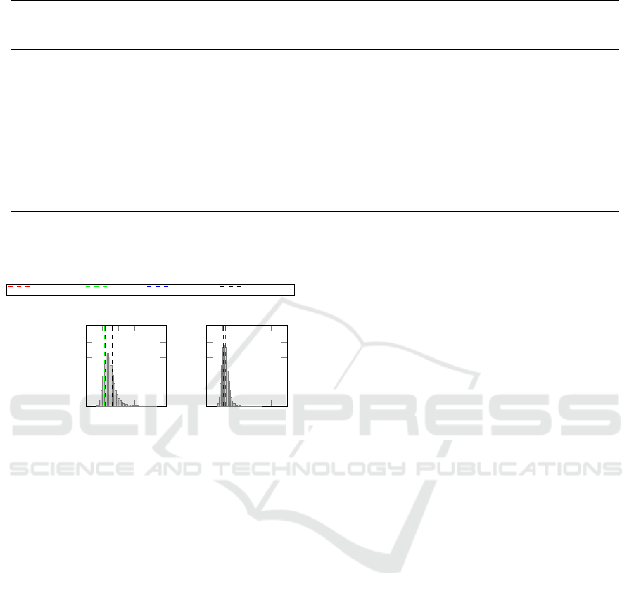
Table 1: Summary of optimization results indicated by the NRMSE.

opt.

type

loss

APRBS

Opt

GOATS

amplitude levels amplitude levels

26 51 101 167 26 51 101 167

SOO

hamm

1st

MAP 0.156 0.105 0.114 0.098 0.137 0.112 0.115 0.114

SAP 0.156 0.111 0.094 0.107 0.136 0.136 0.111 0.109

MSAP 0.136 0.113 0.116 0.101 0.229 0.201 0.140 0.157

AE 0.121 0.116 0.113 0.104 0.114 0.095 0.094 0.098

MP 0.109 0.126 0.092 0.106 0.107 0.103 0.111 0.10

FA 0.127 0.110 0.121 0.115 0.178 0.135 0.084 0.076

wiener

1st

AE 0.147 0.150 0.126 0.138 0.142 0.112 0.106 0.101

hamm

2nd

AE 0.181 0.175 0.156 0.163 0.156 0.144 0.158 0.170

MOO

hamm

1st

AE+MAP 0.097 0.111 0.098 0.103 0.120 0.119 0.105 0.105

AE+SAP 0.146 0.121 0.104 0.110 0.311 0.267 0.214 0.183

AE+MSAP 0.150 0.105 0.104 0.107 0.136 0.175 0.119 0.181

0.1

0.2

0.3

0.4

0.5

400

800

1,200

1,600

2,000

NRMSE

no. models

26 levels

0.1

0.2

0.3

0.4

0.5

400

800

1,200

1,600

2,000

NRMSE

51 levels

APRBS

Opt

GOATS OMNIPUS APRBS

Std

Figure 2: Comparison of the step-based signals with the

histogram of test errors for APRBS

10000

for hamm

1st

tions f

is investigated. The performance of the ex-

citation signals which are optimized according to f

for 26 amplitude levels, is not better than the mean

value of the NRMSE for the APRBS

10000

illustrated

in Fig. 2 and Table 1. It is even sometimes worse than

the mean value of the APRBS

10000

which leads to the

assumption, that f

does not have the main effect on

the model performance. Another point which under-

pins this assumption is that the GOATS optimized ac-

cording to f

result in quite volatile and sometimes

relatively bad model qualities. The reason for this is

the degree of freedom in the sequence of the GOATS

in contrast to the APRBS

Opt

. Due to the degree of

freedom the f

can drive the sequence of the GOATS

to short durations so that the equilibrium is not cov-

ered sufﬁcient. For a higher amount of amplitude lev-

els, the achieved model quality for the APRBS

Opt

and

GOATS optimized according to the f

becomes bet-

ter. This can be explained since the input space will be

covered good enough, if just enough amplitude levels

are modulated.

In addition, all f

also are optimized together with

the AE loss function in a MOO to prove if it can con-

tribute additional information which are not consid-

ered by f

. For these optimizations the modeling per-

formance is in the same range as the modeling quality

of the SOO with f

. Therefore, the optimization ac-

cording to f

does not lead to an improvement of the

modeling quality. The explanation for this is given

by the structure of the step-based signals which limits

the degree of freedom of optimization of the evenly

excitation of all frequencies resulting in too similar

amplitude spectra of the different step-based signals.

For this reason, only the SOO of f

is further consid-

ered for the optimization of the step-based excitation

signals.

Figure 2 shows the comparison of the APRBS

Opt

and GOATS optimized with the loss AE in SOO and

the two state of the art step-based signals OMNIPUS

and APRBS

Std

. The modeling quality achieved by

the different step-based excitation signals is indicated

by the dashed lines. Consider that the APRBS

Std

and the APRBS

Opt

share the same sequence. Fig-

ure 2 indicates that an optimization of the permu-

tation of the APRBS

Opt

compared to the APRBS

Std

leads to an improvement of the modeling quality. Al-

though this improvement is limited due to the de-

gree of freedom of the APRBS

Opt

. This can be an-

alyzed through the comparison of the achieved model

quality of APRBS

Opt

to the quality of the GOATS.

The GOATS exceeds the APRBS

Opt

in all investigated

cases, because it can better cover the space due to

its degree of freedom in the duration of each ampli-

tude level. Consider that similar results are obtained

for the wiener

1st

and hamm

2nd

so they are omitted

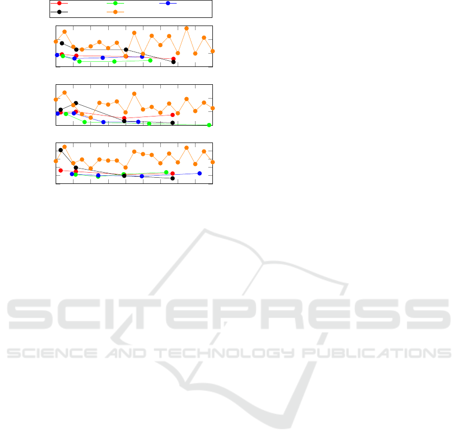
in Fig. 2 to conserve space. Figure 3 illustrates the

comparison of step-based and sinusoid-based signals

over different signal durations for the achieved model

Genetic Optimization of Excitation Signals for Nonlinear Dynamic System Identiﬁcation

143

20 40 60 80 100 120 140 160 180 200

0.08

0.13

0.18

0.23

NRMSE

20 40 60 80 100 120 140 160 180 200

0.1

0.15

0.2

0.25

NRMSE

20 40 60 80 100 120 140 160 180 200

0.1

0.15

0.2

0.25

0.3

0.35

time in s

NRMSE

hamm

1st

wiener

1st

hamm

2nd

APRBS

Opt

GOATS OMNIPUS

APRBS

Std

Multi-Sine

Figure 3: Comparison of test errors for step-based and

sinusoid-based signals over signal duration.

quality on the test data. Comparing the OMNIPUS

to the GOATS, the GOATS has a similar performance

except for the hamm

1st

for the amounts of amplitude

levels 51, 101 and 167 and for the wiener

1st

with 51

points where it surpasses the OMNIPUS more sig-

niﬁcantly. The GOATS is the only excitation signal

which in all cases signiﬁcantly outperforms the mean

values of the APRBS

10000

(17% − 28 %).

The Chirp is omitted of Fig. 3 for better visibility,

but it performs like the Multi-Sine. Figure 3 shows

that the step-based signals signiﬁcantly exceed the si-

nusoid signals in the achievable model quality. Fur-

thermore, the model quality for the different durations

of the sinusoid-based signals is quite volatile. In ad-

dition, the optimized signals like APRBS

Opt

, GOATS

and OMNIPUS clearly outperform all other excitation

signals for short signal durations. For longer signal

durations (approximately 2 − 4 times) the APRBS

Std

can achieve a comparable model quality, because with

enough amplitude levels the space will be covered

good, when the amplitude levels which are modulated

to an APRBS are selected with a space-ﬁlling crite-

rion.

6 CONCLUSION AND OUTLOOK

The current paper proposes two novel approaches

for the optimization of step-based excitation signals

—APRBS

Opt

and GOATS — for nonlinear dynamic

system identiﬁcation. For this purpose, the coverage

of the space spanned by the system’s input and out-

put and the evenly excitation of all frequencies of the

step-based signals have been investigated as objec-

tives for the optimization via a GA. The APRBS

Opt

and GOATS are compared with four state-of-the-art

excitation signals (APRBS

Std

, Chirp, Multi-Sine and

OMNIPUS) on the three artiﬁcially created nonlinear

dynamic processes in order to evaluate the expectable

model quality.

Our results show that the optimization of the

space-ﬁlling coverage of the step-based excitation

signals leads to a signiﬁcant improvement of the

model quality compared to the usage of a APRBS

Std

for short signal durations. The reason for this is the

avoidance of unexplored areas in the space spanned

by the system’s input and output. In contrast to our

expectation, the results show that our optimization

of an evenly distributed amplitude spectrum does not

yield an improvement of the model quality. This can

be explained by the given structure of the step-based

signals which limits the degree of freedom for the op-

timization of the evenly excitation of all frequencies

resulting in too similar amplitude spectra.

Therefore, the single objective optimization of the

uniform coverage of the space is used for our newly

developed excitation signals APRBS

Opt

and GOATS.

The APRBS

Opt

, leads to an improved model qual-

ity compared to the standard APRBS which shares

the same PRBS basis. The improvement is, how-

ever, limited due to its degree of freedom constrained

by the given PRBS. We have found that the GOATS

leads to a signiﬁcantly higher model quality com-

pared to the state-of-art-excitation signals APRBS

Std

Chirp, Multi-Sine and a slightly higher model quality

in comparison to the OMNIPUS on the three investi-

gated artiﬁcial nonlinear dynamic processes. In addi-

tion, the GOATS is suitable for stiff systems, capable

of supplementing existing data and easy incorporation

of constraints.

The present results are limited to the three arti-

ﬁcially created low order dynamical SISO systems.

Therefore, in future research the GOATS has to be in-

vestigated for higher dimensional, higher dynamical

order and real world systems. Another future research

topic is the investigation of new loss functions for the

optimization.

REFERENCES

Audze, P. and Eglais, V. (1977). New approach for plan-

ning out of experiments. Problems of Dynamics and

Strengths, 35:104–107.

Baumann, W., Schaum, S., Roepke, K., and Knaak, M.

(2008). Excitation Signals for Nonlinear Dynamic

Modeling of Combustion Engines. In Proceedings of

ICINCO 2021 - 18th International Conference on Informatics in Control, Automation and Robotics

144

the 17th World Congress The International Federation

of Automatic Control, pages 1066–1067.

Davis, L. (1985). Applying Adaptive Algorithms to

Epistatic Domains. In Proceedings of the 9th Inter-

national Joint Conference on Artiﬁcial Intelligence,

pages 162–164.

Deb, K. and Agrawal, R. B. (1995). Simulated Binary

Crossover for Continuous Search Space. Complex

Systems, 9:115–148.

Deb, K., Agrawal, S., Pratap, A., and Meyarivan, T. (2000).

A fast elitist non-dominated sorting genetic algorithm

for multi-objective optimization: NSGA-II. In Inter-

national conference on parallel problem solving from

nature, pages 849–858.

Deep, K., Singh, K. P., Kansal, M. L., and Mohan, C.

(2009). A real coded genetic algorithm for solv-

ing integer and mixed integer optimization problems.

Applied Mathematics and Computation, 212(2):505–

518.

Deﬂorian, M. and Zaglauer, S. (2011). Design of exper-

iments for nonlinear dynamic system identiﬁcation.

IFAC Proceedings Volumes, 44(1):13179–13184.

Goldberg, D. E. and Deb, K. (1991). A Comparative Analy-

sis of Selection Schemes Used in Genetic Algorithms.

Foundations of genetic algorithms, 1:69–93.

Goldberg, D. E., Lingle, R., and Others (1985). Alleles,

loci, and the traveling salesman problem. In Pro-

ceedings of an international conference on genetic al-

gorithms and their applications, volume 154, pages

154–159.

Hartmann, B. (2013). Lokale Modellnetze zur Identiﬁkation

und Versuchs- planung nichtlinearer Systeme. PhD

thesis, University of Siegen.

Hartmann, S. (1998). A Competitive Genetic Algorithm

for Resource-Constrained Project Scheduling. Naval

Research Logistics (NRL), 45:733–750.

Heinz, T. O. and Nelles, O. (2016). Vergleich von An-

regungssignalen f

ur Nichtlineare Identiﬁkationsauf-

gaben. In Hoffman, F., H

ullermeier, E., and Mikut,

R., editors, Proceedings 26. Workshop Computational

Intelligence, pages 139–158. KIT Scientiﬁc Publish-

ing.

Heinz, T. O. and Nelles, O. (2017). Iterative Excitation Sig-

nal Design for Nonlinear Dynamic Black-Box Mod-

els. Procedia Computer Science, pages 1054–1061.

Heinz, T. O., Schillinger, M., Hartmann, B., and Nelles,

O. (2017). Excitation signal design for nonlinear dy-

namic systems with multiple inputs – A data distribu-

tion approach. In R

opke, K. and G

uhmann, C., edi-

tors, International Calibration Conference - Automo-

tive Data Analytics, Methods, DoE, pages 191–208.

expertVerlag.

Hoagg, J. B., Lacy, S. L., Babu

ska, V., and Bernstein, D. S.

(2006). Sequential multisine excitation signals for

system identiﬁcation of large space structures. In Pro-

ceedings of the American Control Conference, pages

418–423.

Holland, J. H. (1975). Adaptation in natural and artiﬁcial

systems: an introductory analysis with applications to

biology, control, and artiﬁcial intelligence.

Isermann, R. (1992). Identiﬁkation dynamischer Systeme 1.

Springer Verlag.

Isermann, R. (2010). Elektronisches Management mo-

torischer Fahrzeugantriebe. Springer.

Joseph, V. R., Gul, E., and Ba, S. (2015). Maximum projec-

tion designs for computer experiments. Biometrika,

102(2):371–380.

Lin, W. Y., Lee, W. Y., and Hong, T. P. (2003). Adapt-

ing crossover and mutation rates in genetic algo-

rithms. Journal of Information Science and Engineer-

ing, 19:889–903.

Nelles, O. (2006). Axes-Oblique Partitioning Strategies for

Local Model Networks. In IEEE International Sympo-

sium on Intelligent Control, pages 2378–2383. IEEE.

Nelles, O. (2013). Nonlinear system identiﬁcation: from

classical approaches to neural networks and fuzzy

models. Springer Science & Business Media.

Nelles, O. and Isermann, R. (1995). Identiﬁcation of nonlin-

ear dynamic systems - classical methods versus radial

basis function networks. In Proceedings of the Ameri-

can Control Conference, volume 5, pages 3786–3790.

Nouri, N. M., Valadi, M., and Asgharian, J. (2018). Optimal

input design for hydrodynamic derivatives estimation

of nonlinear dynamic model of AUV. Nonlinear Dy-

namics, 92(2):139–151.

Peter, T. J. and Nelles, O. (2019). Fast and sim-

ple dataset selection for machine learning. at-

Automatisierungstechnik, 67(10):833–842.

Pintelon, R. and Schoukens, J. (2012). System identiﬁca-

tion: a frequency domain approach, volume 478. John

Wiley & Sons.

Razali, N. M. and Geraghty, J. (2011). Genetic algorithm

performance with different selection strategiesin solv-

ing TSP. In Proceedings of the World Congress on

Engineering, volume 2, pages 1–6.

Rivera, D. E., Lee, H., Mittelmann, H. D., and Braun, M. W.

(2002). Constrained multisine input signals for plant-

friendly identiﬁcation of chemical process systems.

IFAC Proceedings Volumes, 35(1):425–430.

Sivanandam S.N., D. S. (2008). Introduction to genetic al-

gorithms. Berlin: Springer.

Syswerda, G. (1991). Scheduling optimization using ge-

netic algorithms. Handbook of genetic algorithms.

Tietze, N. (2015). Model-based calibration of engine con-

trol units using gaussian process regression. PhD the-

sis, Technische Universit

at Darmstadt.

Genetic Optimization of Excitation Signals for Nonlinear Dynamic System Identiﬁcation

145