
A Machine Learning Approach for NDVI Forecasting
based on Sentinel-2 Data
Stefano Cavalli
a
, Gabriele Penzotti
b
, Michele Amoretti
c
and Stefano Caselli
d
CIDEA, University of Parma, Parco Area delle Scienze, Parma, Italy
Keywords:
Satellites, Artificial Intelligence, Vegetation Index, Machine Learning, Data Mining.
Abstract:
The Normalized Difference Vegetation Index (NDVI) is a well-known indicator of the greenness of the biomes.
NDVI data are typically derived from satellites (such as Landsat, Sentinel-2, SPOT, Pl
`
eiades) that provide
images in visible red and near-infrared bands. However, there are two main complications in satellite image
acquisition: 1) orbits take several days to be completed, which implies that NDVI data are not daily updated; 2)
the usability of satellite images to compute the NDVI value of a given area depends on the local meteorological
conditions during satellite transit. Indeed, the discontinuous availability of up to date NDVI data is detrimental
to the usability of NDVI as an indicator supporting agricultural decisions, e.g., whether to irrigate crops or not,
as well as for alerting purposes. In this work, we propose a multivariate multi-step NDVI forecasting method
based on Long Short-Term Memory (LSTM) networks. By careful selection of publicly available but relevant
input data, the proposed method has been able to predict with high accuracy NDVI values for the next 1, 2 and
3 days considering regional data of interest.
1 INTRODUCTION
Precision Agriculture (PA) is a whole-farm manage-
ment approach using information technology, satellite
positioning data, remote sensing and proximal data
gathering. PA employs data from multiple sources to
improve crop yield and increase the cost-effectiveness
of crop management strategies including fertilization
and irrigation. The goal is optimizing returns on in-
puts whilst reducing environmental impacts.
In order to implement data-driven PA, suitable
metrics of crop vigor, health, or development are
needed. The Normalized Difference Vegetation Index
(NDVI) is an indicator of the greenness of the biomes.
Its simple formulation is:
NDV I =
ρ
NIR
− ρ
R
ρ
NIR
+ ρ
R
(1)
where ρ
NIR
and ρ
R
are the spectral reflectance mea-
sured in the near-infrared and visible red wavebands
respectively. In the last two decades, the NDVI
has been widely used for ecosystem monitoring and
specifically as a proxy for vegetation vigor, especially
a
https://orcid.org/0000-0002-3505-0556
b
https://orcid.org/0000-0001-5557-6435
c
https://orcid.org/0000-0002-6046-1904
d
https://orcid.org/0000-0003-0774-7871
for crop monitoring in agriculture. Accurate and com-
prehensive NDVI assessment or forecast has been
shown to enable effective future projections of crop
yield for precise agricultural planning and budgeting
(Hatfield et al., 2008; Reddy and Prasad, 2018). In-
deed, NDVI is strongly correlated with green canopy
cover and the greenness of the vegetation.
Satellite-based multispectral imagery is a major
source of data enabling computation of NDVI and
other vegetation indices for large cultivated areas.
However, satellite data are subject to drawbacks lim-
iting direct NDVI applicability in the context of agri-
cultural decision support systems or crop monitor-
ing. Satellite transit above a given area usually oc-
curs every few days or weeks, depending on the spe-
cific satellite, which leads to an intermittent update
of measured NDVI values. Moreover, possible local
cloud cover and other meteorological factors during
satellite transit affect the spectral response, leading to
further missing NDVI values. For these reasons, ac-
curate NDVI forecasting plays a major role for effec-
tive use of NDVI as a reliable indicator.
In the NDVI forecasting literature, two different
levels of precision are typically examined. The first
one, large-area forecast involves a model that pre-
dicts the NDVI over a large, relatively homogeneous
area such as a whole irrigation district or a whole
Cavalli, S., Penzotti, G., Amoretti, M. and Caselli, S.
A Machine Learning Approach for NDVI Forecasting based on Sentinel-2 Data.
DOI: 10.5220/0010544504730480
In Proceedings of the 16th International Conference on Software Technologies (ICSOFT 2021), pages 473-480
ISBN: 978-989-758-523-4
Copyright
c
2021 by SCITEPRESS – Science and Technology Publications, Lda. All rights reserved
473

forest cover. Conversely, field-level forecast uses a
model that attempts to predict the NDVI in smaller
parcels that are comparable to the size of a field.
One or few hectares can serve as a reference size
for field-level NDVI assessment, based on the avail-
able satellite data (e.g., NASA MODIS satellites pro-
vide a pixel resolution of 250m ×250m (Ahmad et al.,
2020)). In both cases, several issues arise when col-
lecting NDVI data for a dataset suitable for training
and testing the models. The major problem is cop-
ing with outliers, i.e., pixels whose NDVI value is
meaningless, due for example to the presence of ob-
stacles between the measurement device and the tar-
get. Consider, e.g., satellite NDVI imagery acquired
in the presence of clouds. On the other hand, field-
level forecasts are more useful to producers, as they
provide more comprehensive information about how
their fields are evolving. Unfortunately, field-level
NDVI is harder to predict, because the NDVI time
series of a field-level pixel is much more noisy than
the time series of the average observed NDVI over a
large area. Another aspect impacting problem com-
plexity is the forecasting horizon: some approaches
only predict the next NDVI value, whereas others aim
at multi-step predictions.
In this paper, we focus on field-level forecast us-
ing very small pixels — at a 10m × 10m resolution.
We propose an LSTM-based forecasting approach
taking into account four features, namely NDVI,
atmospheric precipitation, minimum and maximum
temperature. The proposed forecasting model allows
the prediction of the next k NDVI values, given a time
series of t data items. Each time step corresponds
to one day. The method illustrated in the paper has
shown the ability to predict the NDVI for the next 1,
2 and 3 days with high accuracy, considering a broad
area of cultivated fields in the Emilia-Romagna Re-
gion, Italy.
The paper is organized as follows. In section 2,
we discuss related work on NDVI forecasting. In sec-
tion 3, we provide a detailed problem statement, with
a list of tasks we focus on. In section 4, we illustrate
the proposed approach. In section 5, we present ex-
perimental results. Finally, in section 6, we conclude
the paper with an outline of future work.
2 RELATED WORK
A considerable amount of previous work on the es-
timation of the NDVI of the current growing sea-
son uses traditional time-series forecasting and curve-
fitting techniques (Atkinson et al., 2012; Cao et al.,
2015; Vorobiova and Chernov, 2017). However, these
techniques are outperformed by methods based on
deep learning with time series analysis.
The approach proposed by G
´
omez-Lagos et al.
(G
´
omez-Lagos et al., 2019) utilizes a standard (non-
recurrent) fully connected neural network to predict
the NDVI values of a table grape orchard at the field
level. One of the drawbacks of this methodology is
that it is only tested on the NDVI pixels of one date.
Therefore, these results are not comparable with al-
gorithms that measure their accuracy across multiple
timestamps over a season. The model would need to
be retrained every time an NDVI prediction for a new
date is required.
Given the sequential nature of NDVI forecasting,
another emerging method to forecast NDVI is the use
of an RNN or its variant, the LSTM (Long Short-
Term Memory). Reddy’s methodology (Reddy and
Prasad, 2018) involves using the LSTM to perform
large-area NDVI forecasts and achieves a root mean
square error (RMSE) of less than 0.03. While this is
a low RMSE, this LSTM is forecasting the average
over large areas, which, as mentioned earlier, is an
easier task than field-level predictions. Stepchenko
and Chizhov (Stepchenko and Chizhov, 2015) per-
form single-pixel field-level forecasts at a similarly
low RMSE of 0.0352, but approximately half pixels
in this study contain coniferous vegetation rather than
crop fields. Coniferous regions are significantly easier
to predict than crop areas due to their homogeneous
and regular evolution. Additionally, a smoothing co-
efficient of 15% is used to reduce noise and remove
cloudy data. More recently, Ahmad et al. (Ahmad
et al., 2020) have proposed the ConvLSTM methodol-
ogy to perform field-level multipixel predictions with
an RMSE of 0.0782. In the context of field-level
NDVI forecasting, this result can be considered as the
state of the art. However, (Ahmad et al., 2020) oper-
ate with relatively large 250m × 250m pixels suitable
for large fields typical of Southern American agricul-
ture, whereas we aim at the ability to predict NDVI
even for the more fragmented fields more customary
in Europe.
3 PROBLEM STATEMENT
For a given field, let us consider a sequence of daily
observations, each one consisting of the following
features: NDVI, precipitation level, minimum tem-
perature, maximum temperature. Our goal is to pre-
dict the next k NDVI values — i.e., NDVI(t + 1), ..,
NDVI(t + k) — with high accuracy. For this purpose,
we will use a suitable ML model trained with histori-
cal data.
ICSOFT 2021 - 16th International Conference on Software Technologies
474

As NDVI data sources, we rely upon the Sentinel-
2A and Sentinel-2B satellites, which are part of the
Copernicus Sentinel-2 mission
1
(European Union,
2021). We use the 10m × 10m spatial resolution in
order to increase the accuracy of the NDVI estimation
by providing as much data as possible. Higher spatial
resolutions are also available from other satellites or
services.
Of the aforementioned features, the NDVI one
may have missing values, due to the fact that the satel-
lites do not pass over the given every day. Indeed, the
two satellites provide a 5-day revisiting time within
out-of-phase orbits. Hence, the actual time interval
between the acquisition of a satellite image of a given
plot and the next one is about 2-3 days. Moreover,
when it comes to cloudy weather, the NDVI values
may also be falsified. The cloud coverage problem
has been the subject of several studies (Roerink et al.,
2000) (Alvarez-Mendoza et al., 2019) (Tarrio et al.,
2020).
Thus, we focus on the following tasks:
• Satellite’s near-infrared and visible red bands re-
trieval;
• Cloud detection in cloudy weather conditions for
NDVI validation;
• Weather information retrieval from ARPAE Re-
gional System;
• NDVI regression, i.e., given a multivariate time
series with the aforementioned features, predict
next NDVI value(s).
In the following section, we describe the proposed
approach for coping with these tasks.
4 PROPOSED APPROACH
In our method, two independent subsystems extract
data from the Sentinel-2 Copernicus repository and
from the available weather station, respectively. The
resulting multivariate dataset is used to train an LSTM
regression model, which will be used to predict, given
a t-step input sequence, the next k NDVI values. A
grid search algorithm provides the best hyperparame-
ter configuration.
4.1 Field Data Retrieval
The first step to the construction of the dataset is the
selection and collection of the agricultural fields. We
consider only fields with a regular shape, preferring
polygons with a low number of vertices. As for the
1
https://www.copernicus.eu/en
size, we use only pixels with an area of medium or
high size, distributing the samples in a balanced way
in the range between 10000 and 70000 square meters.
With these choices it is possible to obtain a high num-
ber of satellite pixels, enabling more effective and ro-
bust preprocessing such as cloud removal.
Regarding the geographical position, a reasonable
choice is to exclude fields in the mountain and pre
mountain areas due to the uncertainty of the meteo-
rological data (few weather stations in relation to the
morphology of the terrain) and to the more frequent
presence of cloud formations during the growing sea-
son of the crop (obscuring the field from satellite).
Concerning the cultivation type, we limit the se-
lection to open field, large-scale herbaceous crops,
suitable for a predictive observation of the NDVI
curve from sowing to harvesting.
4.2 Sentinel-2 Satellite Data
The two satellites of the Sentinel-2 mission have a sun
synchronous orbit and together they are able to cover
all the mainland surfaces with a time interval of 5 days
between two revisits. The satellites supply data prod-
ucts of different types organized in tiles of 100x100
km
2
. Due to the overlap between two adjacent or-
bits, some areas have more frequent coverage. For
example, in the case of the Emilia-Romagna region,
coverage is guaranteed by satellite sensing carried out
in orbits 22 and 65 (relative numbers) which enable a
sampling every 2-3 days.
The Sentinel-2 satellite data of interest are the in-
dividual bands needed for computation of the NDVI
index, namely the B8 (NIR) and B4 (RED), and the
Cloud Mask (obtained by ESA’s cloud classification).
For each terrain, we need to obtain the pixel map,
through the intersection of the polygon with the 10m
× 10m resolution products. Finally, an NDVI value
must be calculated and associated with each pixel of
each terrain, using the corresponding values in the B8
and B4 band.
4.3 Map Validation
The obtained values are affected by noise. First, the
data representing the geographical coordinates of the
fields, i.e. the perimeter polygons, are usually man-
ually entered into geographical information systems.
For this reason, in some cases the process involving
this manually inserted data does not exactly reflect the
representation of the position of the field, especially
in the outermost area. For example, they may include
parts of adjacent roads, buildings, or other neighbor-
ing fields. For this reason, we choose to remove all
A Machine Learning Approach for NDVI Forecasting based on Sentinel-2 Data
475
the border pixels within each field.
Another source of uncertainty is related to the geo-
referencing of satellite data. As described in an offi-
cial ESA quality report (ESA, 2021), calibration of
satellites is constantly evolving in order to improve
accuracy: the last calibration for Sentinel-2B was per-
formed on March 30th, 2020, whereas the geoloca-
tion performance of Sentinel-2A has remained good
since the last calibration in January 2019. According
to ESA, provided data may be affected by an error,
due to satellite vibration and oscillation, of about 10
m in the worst case.
In order to limit the impact of these errors, we
propose to weigh the values based on the pixel po-
sition, considering the central pixels as more repre-
sentative of the crop status than those located close
to the border. Accordingly, the latter pixels receive
a lower weight than the former ones. The closer one
gets to the center of the field, the higher is the weight
of pixels.
Table 1: Example of linearly increasing pixel weight levels.
L
0
L
1
L
2
L
3
L
4
0.00 0.25 0.50 0.75 1.00
Table 1 defines five levels for the pixel weights,
which grow linearly from 0 to 1. In general, we de-
note the set of pixel weight levels as
L = {L
0
, L
1
, L
2
, L
3
, L
4
}. (2)
4.4 Cloud Detection for NDVI
Validation
Cloud detection is one of the critical points in the
analysis of satellite images. Since the NDVI value is
very sensitive to cloudy, foggy and rainy weather con-
ditions, the images cannot be analyzed without con-
sidering all these meteorological factors.
In cloudy conditions, the NDVI value turns out
to be close to 0, sometimes even negative (Lillesand
et al., 2015). Considering that water has a uniform
and low reflectance in the near-infrared, cloud detec-
tion in such environment is much easier, while it is
more difficult over land.
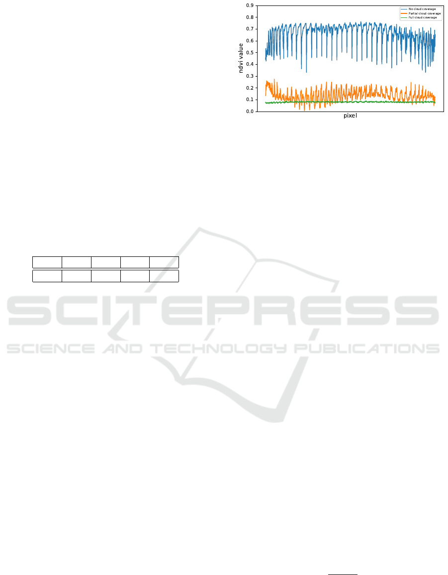
An example set of pixel-related NDVI values in
different weather conditions is reported in Figure 1.
The NDVI value is close to 0 in those pixels where
the crop field is not clearly visible, while it continue
to grows as the clouds disappear.
This type of analysis must be repeated for all con-
sidered fields. We propose to apply a clustering al-
gorithm to separate pixels with high visibility from
pixels with low visibility. The latter pixels must be
Figure 1: NDVI values for each 10m × 10m pixel in case
of no cloud coverage (blue), partial cloud coverage (orange)
and full cloud coverage (green).
removed, otherwise they would be detrimental to the
final model performance.
The main difference in using a fine-grained ap-
proach (with small pixels) instead of a coarse-grained
one is that the former enables the selective removal
of the outliers. For example, within a 250m × 250m
pixel, some of its 10m × 10m subpixels may have a
wrong value (due to clouds or fog) while some others
may have correct values. Instead of removing the en-
tire large pixel, we propose to reject just those where
the NDVI value is below a threshold α that can be
estimated by means of the aforementioned clustering
process. As mentioned in Section 4.2, for cloud mask-
ing we propose an adaptation of the homonym ser-
vice offered by Sentinel. Indeed, that service detects
most of the clouds but not all of them. For this rea-
son, we combine a more selective algorithm alongside
the Sentinel one in order to recognize more precisely
where the clouds are located.
Based on the percentage and position of the
cloudy pixels, we propose a method that can discrim-
inate the crop’s validity. Let us denote as P the set of
field pixels:
P = {p
1
, p
2
, ..., p
|P |
}. (3)
The weighted number of pixels classified as cloudy,
according to the threshold we mentioned earlier, is
denoted as
n
+
=
|P |
∑
i=1
ndvi
i
<α
w
i
, (4)
where w
i
∈ L and ndvi
i
is the NDVI value of the pixel
p
i
.
We define the weighted cloud coverage percentage
as
ccp =
n
+
∑
|P |
i=1
w
i
· 100, (5)
which represents the percentage of cloudy pixels
within a field, based on their weights. A field is ac-
cepted if its ccp does not exceed 25%.
ICSOFT 2021 - 16th International Conference on Software Technologies
476
When the cloud detection algorithm identifies a
cloudy field or the satellites do not pass over a field,
we propose to perform a linear NDVI interpolation
in order to preserve the dataset consistency. Based
on these considerations, the weighted average NDVI
value for a given field f and day d is thus defined as
ndvi
f ,d
=
∑
|P |
i=1
ndvi
i
· w
i
∑
|P |
j=1
w
j
. (6)
4.5 Weather Information Retrieval
In order to manage the lack of NDVI values during the
days where satellites did not pass over the fields, or
just found bad climatic conditions, we propose to take
into account other variables. In particular, the amount
of precipitation, the minimum temperature and the
maximum temperature, together with the NDVI in-
dex, are part of the considered dataset. Temporal cor-
relations between NDVI index, temperature and pre-
cipitation have been extensively studied (Ichii et al.,
2002) (Piao et al., 2006) in the last decades.
Taking advantage of the 10m × 10m pixels pre-
viously defined, our approach avoids a one-by-one
weather station with crop field assignment. Indeed,
our algorithm makes multiple weighted average as-
signments between neighboring weather stations and
each pixel.
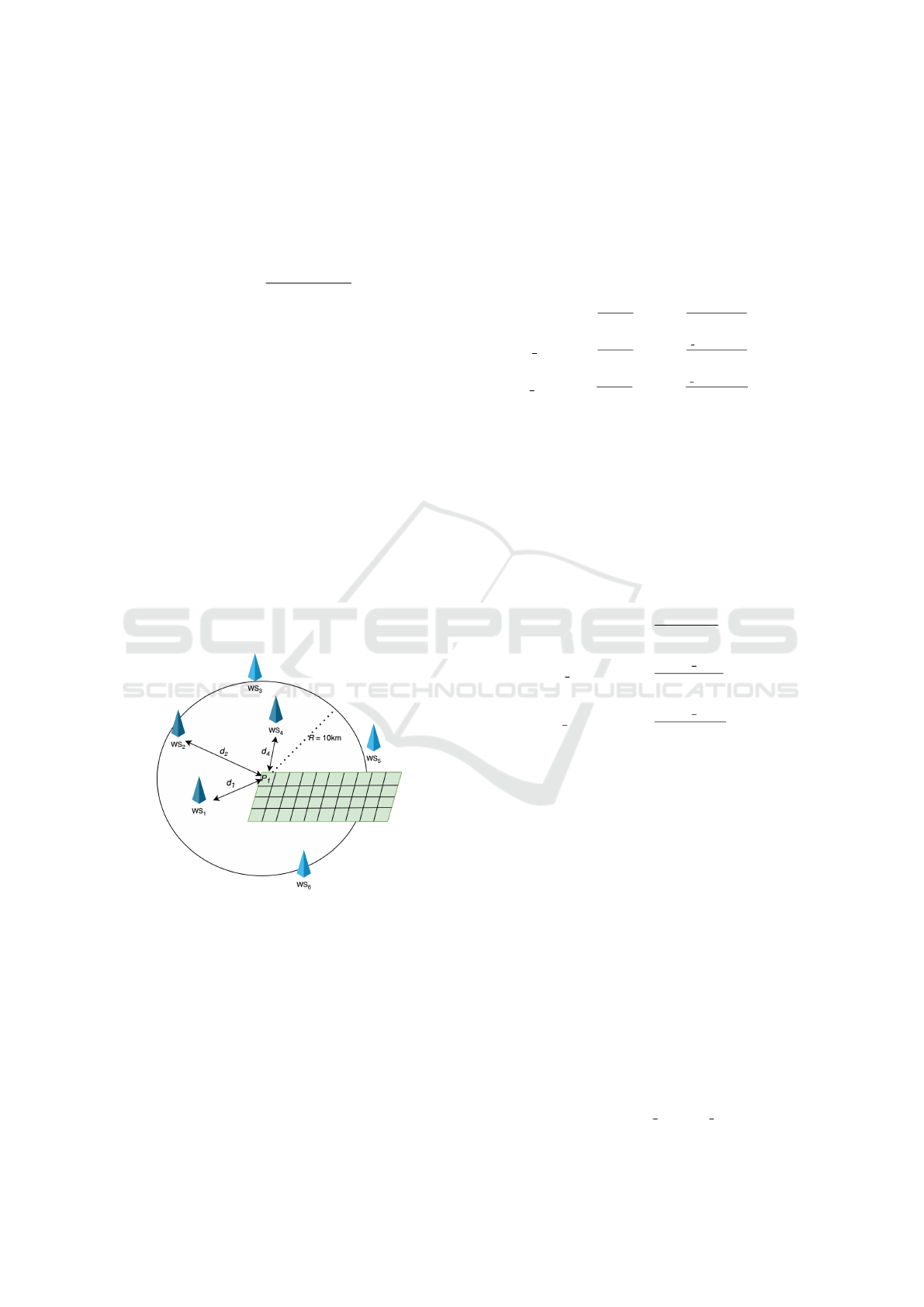
Figure 2: Weighted average of the information provided by
the weather stations (ws) based on their distance (d), for
a given pixel (P
1
) within a circle centered on P
1
of radius
R=10km.
Figure 2 schematizes the algorithm that assigns
the values of precipitations, minimum temperature
and maximum temperature to a pixel of a specific
field. Considering the set of pixels P (eq. 3), the cir-
cular region of radius R that surrounds the i-th pixel
p
i
is
C
i
= {(lat, lon) : (lat − lat
i
)
2
+ (lon − lon
i
)
2
< R
2
}
(7)
where (lat
i
, lon
i
) are the geographical coordinates of
the centroid of p
i
. The set of the weather stations that
belong to C
i
is
W
i
= {ws : (lat
ws
, lon
ws
) ∈ C
i
}. (8)
Finally, we list the formulas for calculating the pre-
cipitation level, minimum temperature and maximum
temperature related to p
i
:
prec
i
=
w
i
∑
|P |
i=1
w
i
∑
ws∈W
i
prec
ws
·d
ws,i
∑
ws∈W
i
d
ws,i
(9)
t min
i
=
w
i
∑
|P |
i=1
w
i
∑
ws∈W
i
t min
ws
·d
ws,i
∑
ws∈W
i
d
ws,i
(10)
t max
i
=
w
i
∑
|P |
i=1
w
i
∑
ws∈W
i
t max
ws
·d
ws,i
∑
ws∈W
i
d
ws,i
(11)
where d
ws,i
is the distance between the ws position and
the centroid of p
i
. The distance is calculated using the
spherical law of cosines as
d
ws,i
= arccos((sin (lat
ws
) · sin (lat
pi
) +
cos(lat
ws
) · cos (lat
p
i
) · cos (lon
p
i
− lon
ws
)), (12)
in order to deal with geodetic coordinates. The av-
erage precipitation level, minimum temperature and
maximum temperature of a given field f and day d
are defined as
prec
f ,d
=
∑
|P |
i=1
prec
i
|P |
(13)
t min
f ,d
=
∑
|P |
i=1
t min
i
|P |
(14)
t max
f ,d
=
∑
|P |
i=1
t max
i
|P |
. (15)
4.6 Dataset Definition
The set of considered fields is denoted as
F = { f
1
, f
2
, ..., f
|F |
}. (16)
Let us define
D = {D
1
, D
2
, ..., D
|F |
}. (17)
where
D
i
= {d
1
, d
2
, ..., d
|D
i
|
} (18)
is the set of available daily data for a specific field.
Therefore, in order to train a ML model that has
an input sequence of length t and an output sequence
of length k, the following dataset must be used:
X
t,k
= {x
f ,1
, .., x
f ,t
, ndvi
f ,t+1
, .., ndvi
f ,t+k
} (19)
considering all sequences of daily data of length t + k
in D
f
, assuming that |D
f
| ≥ t + k, for all f ∈ F . In
eq. 19, the multivariate data item is a tuple
x
f ,d
= (ndvi
f ,d
, prec
f ,d
,t min
f ,d
,t max
f ,d
). (20)
A Machine Learning Approach for NDVI Forecasting based on Sentinel-2 Data
477
4.7 NDVI Regression
Since a multivariate time series must be processed in
order to forecast NDVI values, we have adopted a
LSTM network (Hochreiter and Schmidhuber, 1997),
using a supervised learning approach. The LSTM net-
work is a special case of recurrent neural network
(RNN) architecture developed to deal with the ex-
ploding and vanishing gradient problems that can be
encountered when training traditional RNNs.
5 EXPERIMENTAL RESULTS
We have evaluated the proposed approach using
Sentinel-2 data referred to the province of Parma in
the Emilia-Romagna region in Italy. Each consid-
ered cultivated field has been uniquely identified by
the triple including geographical position, cultivated
crop, and year. Crop history has been provided by the
Canale Emiliano-Romagnolo (CER) Irrigation Con-
sortium.
Data retrieval has focused on the four years from
2017 (launch year of the Sentinel-2B satellite) to
2020. For each year, we selected 600 fields, for which
we have collected the perimeter polygon (using the
WGS84 coordinate systems) and the reference of the
cultivated crop.
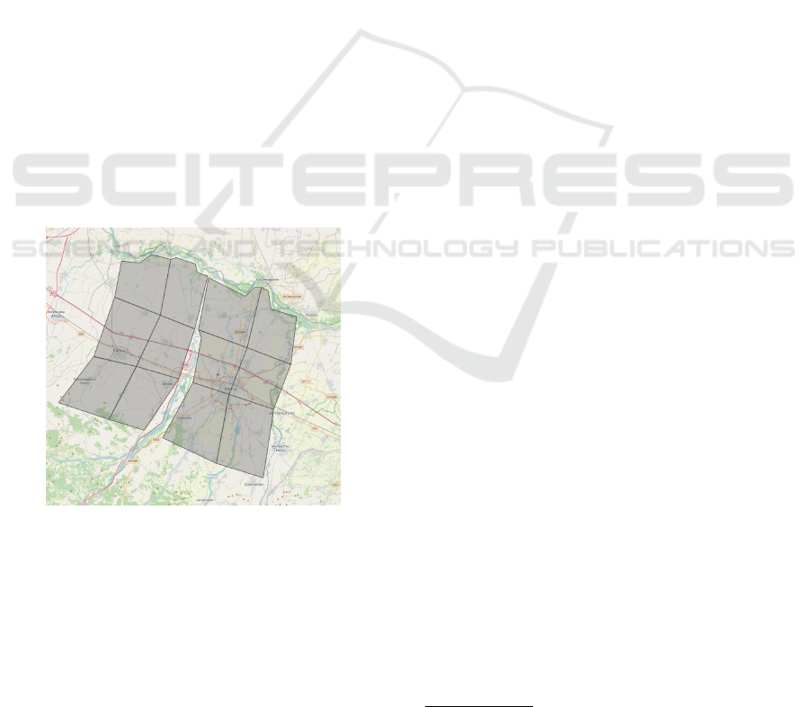
Figure 3: Polygons representing areas of interest during
fields selection.
A balanced selection of the fields has been made
within the sectors shown in Figure 3, which together
represent an area of about 1200 square kilometers. In
particular, fields have been equally chosen from three
crops as follows: tomato, potato and corn. Indeed
the selected crops, in addition to being very relevant
from a food and economic point of view in the region
(Unioncamere Emilia-Romagna and Regione Emilia-
Romagna, 2020), allowed us to obtain, for each year,
a good number of balanced samples in the various cul-
tures and sizes chosen.
Data obtained from the Sentinel-2 satellites have
shown some outliers or inconsistencies, most of the
times due to maintenance, with consequent informa-
tion loss. However, compared with the total amount
of retrieved data, the missing part is relatively small
and can be neglected. The chosen time frame starts on
1st of June and ends on 30th of September (in order to
fully follow the ripening cycle of the chosen crops) for
each of the following four years: 2017, 2018, 2019,
2020.
Each field has been analyzed with a clustering al-
gorithm in order to distinguish between useful NDVI
values and outliers. The result of this analysis is
the threshold value of 0.177, below which the pixel
is considered as an outlier, i.e., a cloudy pixel. In
this way, also thanks to the contribution of the Sen-
tinel cloud detection algorithm, the dataset has been
cleaned in a preprocessing phase that removed about
4.6% of the collected fields.
As already highlighted in Section 4.3, the pro-
posed method assigns different weights to each pixel,
according to its incidence within the field. These
weights are then used to calculate the field’s weighted
cloud percentage: if more than 25% of the pixels, ac-
cording to their impact, are classified as cloudy on a
given day, the field is discarded. To calculate the av-
erage field NDVI value, the same approach based on
pixel weights has been considered.
Meteorological data have been also acquired in the
same time range described above. We have looked
for the largest number of weather stations within the
province of Parma (Emilia-Romagna, Italy) in order
to assign to every 10m × 10 pixel a value of precipi-
tation, minimum temperature, maximum temperature
and NDVI. ARPAE, the agency for prevention, envi-
ronment and energy of Emilia-Romagna region, con-
trols the state of the environment and supports the sus-
tainability of human activities, aiming a the protection
of human health and territorial competitiveness. The
ARPAE Open Data
2
public service allowed us to ex-
tract useful data about weather stations, precipitations
and temperatures of the regional territory. Combin-
ing the completeness of ARPAE Open Data with the
availability of 3Bmeteo
3
historical data, we have been
able to associate at least one weather station for each
of the 44 municipalities within the province of Parma.
Furthermore, some of these municipalities (depend-
ing on their size and geographical location) have been
associated to more than one weather station for a total
of 62.
2
https://dati.arpae.it
3
https://www.3bmeteo.com
ICSOFT 2021 - 16th International Conference on Software Technologies
478
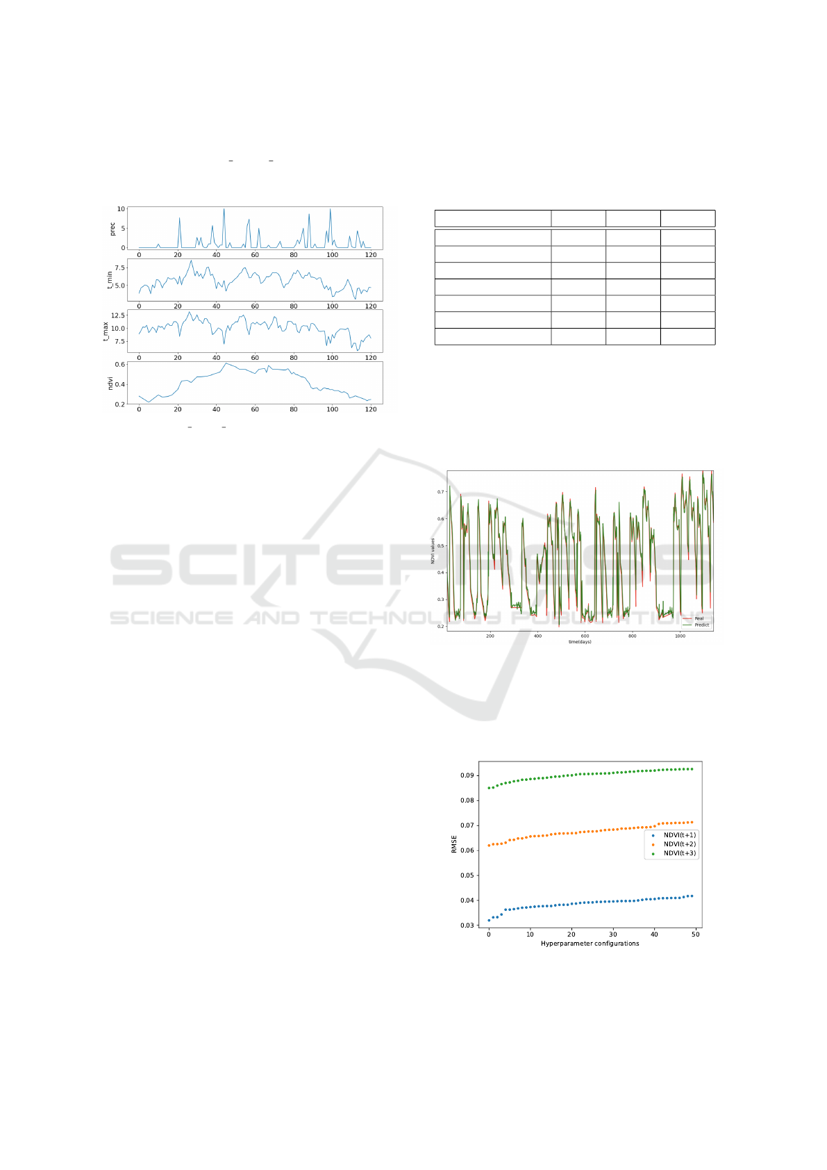
Thus, we have been able to design a dataset with
four features: prec, t min, t max and ndvi. Their
strong correlation is shown in Figure 4, which is re-
lated to a 120-day time range, for a specific field.
Figure 4: prec, t min, t max and ndvi time series example
within a time range of 120 days for a given field.
Model weights are initialized to small random val-
ues and updated by an optimization algorithm in re-
sponse to error estimates on the training dataset. In
particular, we have used the Adam optimizer (Kingma
and Ba, 2015; Sun et al., 2020). Adam is quite dif-
ferent from stochastic gradient descent, which main-
tains a single constant learning rate for all the weights
without updating it during the training phase. In-
stead, Adam benefits from AdaGrad and RMSProp
optimization algorithms that both use a per-parameter
learning rate.
The problem of scaling variable is well known:
unscaled input variables may bring to slow or even
unstable learning process. Exploding gradients can
also appear within regression problems when it comes
to unscaled variables. Therefore, data preparation in-
cludes a pre-processing phase that consists of input
scaling between 0 and 1.
Experiments have been carried out using a work-
station with an Intel Core i9 2.80 GHz CPU, 32 GB
RAM and an NVIDIA GeForce RTX 3090 GB GPU.
The ML software has been implemented in Python 3,
using Keras library with TensorFlow backend.
We have focused on a multi-step time series
forecasting where NDVI(t + 1), NDVI(t + 2) and
NDVI(t + 3) values are predicted. For this task, 20
different experiments have been made by changing
the input time step range from 1 to 20 days back. Con-
sidering (eq. 19), t ranges from 1 to 20, and k = 3.
Finally, the dataset has been partitioned with 60% for
training, 20% for validation and 20% for testing. By
means of a grid search algorithm, we have found that
the parameters and hyperparameters shown in Table
2 are the best possible choices, dealing with a 1-layer
LSTM architecture.
Table 2: Best parameters and hyperparameters values ac-
cording to the grid search algorithm, performed for NDVI
forecasting at days (t +1), (t + 2) and (t +3).
Parameters t + 1 t + 2 t + 3
days back 2 2 3
lstm units 60 105 100
number of epochs 43 116 134
batch size 256 256 64
learning rate (mu) 0.0005 0.0005 0.0005
loss function MAE MAE MAE
optimization alg. Adam Adam Adam
An example of the real NDVI(t + 1) compared
to the NDVI(t + 1) prediction is shown in Figure
(5). The best models that predict NDVI at time
(t +1), (t +2) and (t +3) achieve a RMSE of 0.03189,
0.06201, 0.08506, respectively, thus outperforming
the (Ahmad et al., 2020) ConvLSTM model whose
RMSE stands at 0.0782.
Figure 5: Example of predicted NDVI(t + 1) (green) com-
pared to real NDVI(t + 1) (red).
In Figure (6), we show the per-horizon RMSE of
the most accurate LSTM models we obtained, ordered
from the best model to the worst one.
Figure 6: RMSE result of the first 50 best hyperparameters
configurations.
A Machine Learning Approach for NDVI Forecasting based on Sentinel-2 Data
479

6 CONCLUSIONS
In this work, we have described a novel LSTM-based
approach for NDVI forecasting. In particular, we have
proposed a methodology for building a dataset whose
entries are characterized by weather information and
NDVI values, and a cloud detection algorithm which
refines the one used by the Sentinel-2 Copernicus
mission. Weather information is directly correlated
to the pixels based on their distance, rather than to the
field, in order to increase precision and accuracy of
the dataset by keeping consistency.
In future work, we plan to adopt the new Mis-
tral Data Hub national platform, which provides me-
teorological data related to the whole Country. Fur-
thermore, we plan to implement a parallel system for
satellite image acquisition, to obtain a larger number
of fields in less time. Finally, we will consider alter-
native vegetation indices, such as the Enhanced Vege-
tation Index (EVI), to improve vegetation monitoring
and crop assessment.
SOURCE CODE AND DATASETS
The source code of the proposed LSTM network and
the training data are available on GitHub: https://
github.com/ML-unipr/ndviforecastingML.
ACKNOWLEDGEMENTS
This research was supported by the POSITIVE
project (European Regional Development Fund POR-
FESR 2014-2020, Research and Innovation of the
Region Emilia-Romagna, CUP D41F18000080009).
We thank Canale Emiliano-Romagnolo (CER) Irriga-
tion Consortium for providing data related to fields
and crops of the province of Parma.
REFERENCES
Ahmad, R., Yang, B., Ettlin, G., Berger, A., and Rodr
´
ıguez-
Bocca, P. (2020). A machine-learning based ConvL-
STM architecture for NDVI forecasting. International
Transactions in Operational Research.
Alvarez-Mendoza, C. I., Teodoro, A., and Ramirez-Cando,
L. (2019). Improving ndvi by removing cirrus clouds
with optical remote sensing data from landsat-8 – a
case study in quito, ecuador. Remote Sensing Appli-
cations: Society and Environment, 13:257 – 274.
Atkinson, P., Jeganathan, C., Dash, J., and Atzberger, C.
(2012). Inter-comparison of four models for smooth-
ing satellite sensor time-series data to estimate veg-
etation phenology. Remote Sensing of Environment,
123:400–417.
Cao, R., Chen, J., Shen, M., and Tang, Y. (2015). An im-
proved logistic method for detecting spring vegetation
phenology in grasslands from modis evi time-series
data. Agricultural and Forest Meteorology, 200:9–20.
ESA (2021). S2 MPC - L1C Data Quality Report.
European Union (2021). Copernicus: European Union’s
Earth Observation Programme.
G
´
omez-Lagos, J., Gonz
´
alez-Araya, M., Ortega-Blu, R., and
Espejo, L. (2019). Using data mining techniques to
forecast the normalized difference vegetation index
(ndvi) in table grape. In ICORES 2019.
Hatfield, J., Gitelson, A., Schepers, J., and Walthall,
C. (2008). Application of spectral remote sens-
ing for agronomic decisions. Agronomy journal,
100(3):S117—S131.
Hochreiter, S. and Schmidhuber, J. (1997). Long short-term
memory. Neural Comput., 9(8):1735–1780.
Ichii, K., Kawabata, A., and Yamaguchi, Y. (2002). Global
correlation analysis for ndvi and climatic variables
and ndvi trends: 1982-1990. International Journal
of Remote Sensing, 23(18):3873–3878.
Kingma, D. P. and Ba, J. (2015). Adam: A method for
stochastic optimization. In ICLR 2015.
Lillesand, T., Kiefer, R., and Chipman, J. (2015). Remote
Sensing and Image Interpretation. Wiley.
Piao, S., Mohammat, A., Fang, J., Cai, Q., and Feng, J.
(2006). Ndvi-based increase in growth of temper-
ate grasslands and its responses to climate changes in
china. Global Environmental Change, 16(4):340–348.
Reddy, D. S. and Prasad, P. R. C. (2018). Prediction of
vegetation dynamics using NDVI time series data and
LSTM. Modeling Earth Systems and Environment,
4:409 – 419.
Roerink, G. J., Menenti, M., and Verhoef, W. (2000). Re-
constructing cloudfree ndvi composites using fourier
analysis of time series. International Journal of Re-
mote Sensing, 21(9):1911–1917.
Stepchenko, A. and Chizhov, J. (2015). Ndvi short-term
forecasting using recurrent neural networks. In Proc.
of the 10th Int.l Scientific and Practical Conference.
Sun, S., Cao, Z., Zhu, H., and Zhao, J. (2020). A sur-
vey of optimization methods from a machine learn-
ing perspective. IEEE Transactions on Cybernetics,
50(8):3668–3681.
Tarrio, K., Tang, X., Masek, J. G., Claverie, M., Ju, J., Qiu,
S., Zhu, Z., and Woodcock, C. E. (2020). Comparison
of cloud detection algorithms for sentinel-2 imagery.
Science of Remote Sensing, 2:100010.
Unioncamere Emilia-Romagna and Regione Emilia-
Romagna (2020). Il sistema agro-alimentare
dell’Emilia-Romagna. Technical report.
Vorobiova, N. and Chernov, A. (2017). Curve fitting of
modis ndvi time series in the task of early crops iden-
tification by satellite images. Procedia Engineering,
201:184–195.
ICSOFT 2021 - 16th International Conference on Software Technologies
480
