The Furtherance of Autonomous Engineering via Reinforcement

Learning

Doris Antensteiner

, Vincent Dietrich

and Michael Fiegert

Siemens Technology / Siemens AILab, Munich, Germany

Keywords:

Autonomous Engineering, Reinforcement Learning, Artiﬁcial Intelligence, Industrial Robotics, 6D Pose

Estimation, Computer Vision.

Abstract:

Engineering efforts are one of the major cost factors in today’s industrial automation systems. We present

a conﬁguration system, which grants a reduced obligation of engineering effort. Through self-learning the

conﬁguration system can adapt to various tasks by actively learning about its environment. We validate our

conﬁguration system using a robotic perception system, speciﬁcally a picking application. Perception systems

for robotic applications become increasingly essential in industrial environments. Today, such systems often

require tedious conﬁguration and design from a well trained technician. These processes have to be carried

out for each application and each change in the environment. Our robotic perception system is evaluated on

the BOP benchmark and consists of two elements. First, we design building blocks, which are algorithms and

datasets available for our conﬁguration algorithm. Second, we implement agents (conﬁguration algorithms)

which are designed to intelligently interact with our building blocks. On an examplary industrial robotic

picking problem we show, that our autonomous engineering system can reduce engineering efforts.

1 INTRODUCTION

Continuously increasing need for autonomous and

dynamic industrial production lines leads to an ongo-

ing spread of robotic solutions as well as an increas-

ing requirement for autonomous robotic interactions.

State of the art industrial robotic systems are conﬁg-

ured manually by experienced and trained engineers.

Our goal is to solve robotic engineering tasks auto-

matically, by learning optimized solutions for each

environment. We do this by implementing learning

algorithms and utilizing common interfaces such as

the OpenAI Gym toolkit (Brockman et al., 2016) to

interact with our environment in a standardized way.

This enables an effortless exchange of learning algo-

rithms independent of the environment. To evaluate

our robotic perception system, we are utilizing the

publicly available and commonly used BOP bench-

mark (Hoda

n et al., 2020).

As an applicable precedent for industrial robotic

engineering tasks, we designate robotic picking prob-

lems to be well suited. Finding optimal 6D object

https://orcid.org/0000-0003-2083-0135

https://orcid.org/0000-0003-0568-9727

https://orcid.org/0000-0002-6371-6394

poses (consisting of the object’s position and orienta-

tion in a 3D space) in a scene for industrial robotic

picking applications is essential and has been devel-

oped rapidly in recent history. Not only does this tech-

nology offer a vast ﬁeld of applications, it has also

been shown to be successful enough to lift future bur-

dens in industrial settings. Nevertheless, today such

systems still bear a major challenge, which is the need

of adaption and conﬁguration to the task by a trained

engineer. This process is time consuming and expen-

sive. Therefore, we are introducing a novel approach

for the furtherance of autonomous engineering. By

utilizing learning techniques, we instigate the robots

autonomous adaption to new and challenging situa-

tions, such as different environments, objects, reﬂec-

tion types, occlusions, shadows, illumination or ob-

ject surface structures.

Applications for our approach lie in the ﬁeld of

robotic picking in industrial environments of multiple

ordered or unordered objects with challenging surface

structures (textureless / highly reﬂective), object han-

dling from industrial linear transport lines as well as

assembly tasks.

Antensteiner, D., Dietrich, V. and Fiegert, M.

The Furtherance of Autonomous Engineering via Reinforcement Learning.

DOI: 10.5220/0010544200490059

In Proceedings of the 18th International Conference on Informatics in Control, Automation and Robotics (ICINCO 2021), pages 49-59

ISBN: 978-989-758-522-7

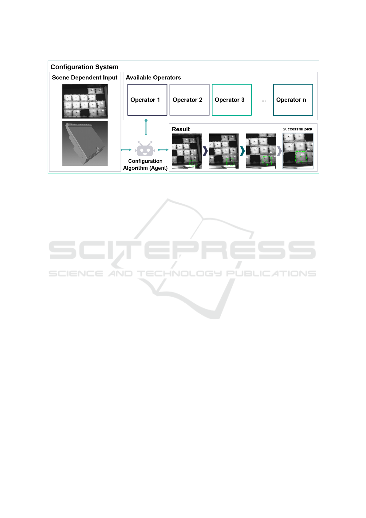
Figure 1: Illustration of the conﬁguration system on an exemplary task. The conﬁguration algorithm (agent) chooses operators

out of a given set, considering the scene input data (input images and object models) and generates a resulting pipeline. Green

lines on the result images indicate the currently estimated position of the object. In this pipeline, operators are chosen to reﬁne

the estimated 6D object pose, until a successful pick is achieved by the robot.

1.1 Contribution

Our approach combines two elements. First, we trans-

fer the operative elements (in our case the 6D pose es-

timation, reﬁnement and scoring functions, as well as

the datasets) into formally modeled building blocks.

This is needed for generating well-designed inter-

faces, which are essential for our conﬁguration algo-

rithm to function properly. Second, we apply the con-

ﬁguration algorithms (being categorized as: hypothe-

sis generation, hypothesis reﬁnement and hypothesis

scoring). We demonstrate a set of learning approaches

(including reinforcement learning and an evolution-

ary method), which interact with our formally mod-

eled blocks, utilizing the standardized interfaces as

deﬁned by the OpenAI Gym toolkit. The main contri-

butions of this paper comprise:

• A systematic organization of our procedural

knowledge in the form of building blocks as well

as suitable interfaces for perception tasks.

• The evaluation of conﬁguration algorithms which

interact with our building blocks.

• A thorough investigation of the interaction of our

conﬁguration algorithms with our building blocks

and the evaluation of all interacting elements with

a focus on the task of 6D pose estimation for in-

dustrial robotic applications.

2 RELATED WORK

In this work, three essential elements are combined

together. First, for our speciﬁc demonstrative appli-

cation, 6D pose estimation algorithms are utilized to

solve robotic picking tasks in simulation. Second, the

conﬁguration elements, including the 6D pose estima-

tion algorithms as well as different datasets, are de-

scribed as formally modeled building blocks in order

to allow for a standardized interaction. Third, learn-

ing algorithms interact with those building blocks

through a standardized interface (where we chose

OpenAI Gym). In this section we present the related

work of each of those elements.

2.1 Robust 6D-Pose Estimation

Fast and robust image-based object detection algo-

rithms are essential for industrial robotic picking

pipelines. Various algorithms were introduced in the

past, each having individual beneﬁts and drawbacks.

Some algorithms show high robustness, but only for

textured and Lambertian objects (Lowe, 2004; Sun

et al., 2011; Yeh et al., 2009). Lambertian objects

exhibit ideal diffuse reﬂection and are well-studied.

More complex challenges can be targeted in various

ways. A popular approach is the use of depth sensors

and RGB-D cameras (Choi and Christensen, 2016;

Tang et al., 2012; Song et al., 2017) to ﬁnd a stable so-

lution. Using multi-view imaging, a non-Lambertian

reﬂection can be suppressed during computation by

enforcing a Lambertian estimation, which is robust

ICINCO 2021 - 18th International Conference on Informatics in Control, Automation and Robotics

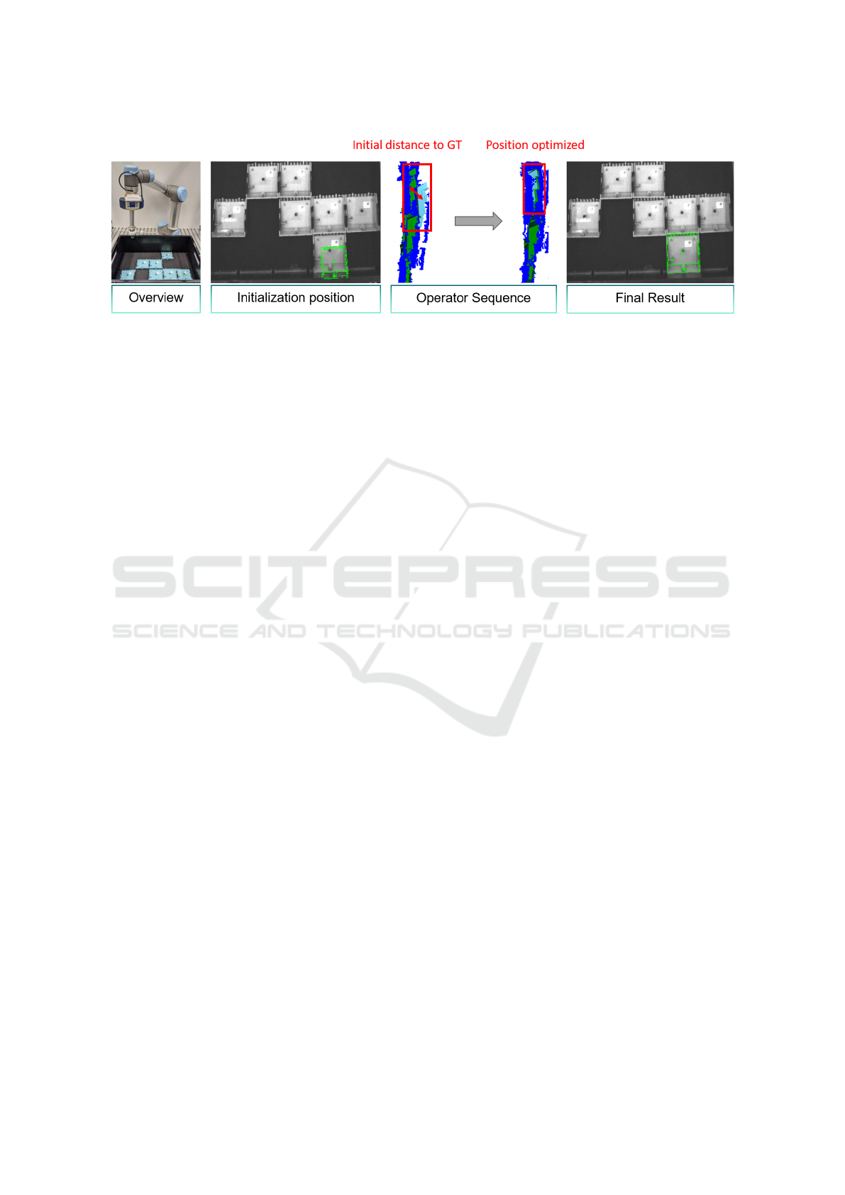
Figure 2: Picture from the view of the robotic arm and a 3D point-cloud illustration from a side view. Shown from both the

initial position as well as the optimized position which results in a successful pick.

to outliers (Hailin Jin et al., 2003). This approach

got special attention in the ﬁeld of light ﬁeld imag-

ing (Wanner and Goldluecke, 2013). Photometric

stereo can be used to model higher order reﬂections

by placing multiple light sources in a systematic po-

sition towards the scene (Chen et al., 2020).

Many such approaches are complementary to each

other and are applicable in special environments (e.g.

high depth variations, symmetries, surface reﬂec-

tions). We demonstrate a formal modeling structure,

which allows for dynamic combinations of various al-

gorithms and hence enables the selection of the op-

timal combination of algorithms for each individual

problem (e.g. unordered and highly reﬂective objects

in a bin together with symmetric matte samples).

2.2 Hierarchical Modeling

Human engineers perform hierarchical tasks given

their prior experience and ability to reason by taking

a sequence of actions. This is a complex process and

enables taking abstract decisions even for unknown

environments. To achieve this with a conﬁguration

algorithm, abstract models are required to translate

these sets of actions to well-deﬁned executable rou-

tines.

For these action spaces, hierarchical planning can

be used to ﬁnd optimal results. While for small action

spaces, a simple search or brute-force approach can

ﬁnd a sufﬁcient solution, hierarchical planning can be

used to ﬁnd improved solutions for large action spaces

and/or time consuming action evaluations. In such

cases a simple search would not succeed. Therefore, a

large problem is factorized and abstracted with a self-

deﬁned model. For our problem, we reduce the action

space by a different approach. Instead of using self-

deﬁned models, we learn models for an abstraction

layer in order to take successful steps in large or costly

action spaces.

Prior knowledge of human engineers can be inter-

preted as strategically developed intuition about the

behavior and use of building blocks, which are easy

and cheap to simulate. We connect such blocks in

the best prior estimated way (e.g. use the most ef-

ﬁcient sequence of optimizers) in order to fulﬁll a

speciﬁc goal (e.g. pick an object with an industrial

robot). By utilizing the hierarchical modeling struc-

ture demonstrated in (Kast et al., 2019), we provide

standardized interfaces for a structured management

of 6D hypothesis generation, reﬁnement and scoring

operations. This permits us to use and combine differ-

ent approaches (blocks) for planing, learning as well

as ﬁnding optimal solutions.

2.3 Learning Algorithms

We utilize machine learning approaches on the exam-

ple of robotic picking solutions, where the learning

algorithms automatically conﬁgures and reﬁnes pa-

rameters for a given scene. Industrial tasks of such

nature are today still solved by human engineers. Our

approach will allow for a faster deployment and re-

duce the required ongoing engineering efforts. Such

directions of industrial robotic automation were pre-

viously discussed in e.g. (El-Shamouty et al., 2019;

Kleeberger et al., 2020).

Our conﬁguration algorithm decides which action

(e.g. a speciﬁc optimization algorithm) to perform

next in a given situation (e.g. pick a metallic item

from an unordered box). We are demonstrating this

by implementing conﬁguration algorithms such as re-

inforcement learning algorithms and evolutionary ap-

proaches.

Previously, automatic decision making for large

action spaces in unknown environments was targeted

by approaches such as AutoML (Hutter et al., 2018).

AutoML makes machine learning more accessible by

reducing the need of human expertise. It takes a

dataset, optimization metric and constraints as input

The Furtherance of Autonomous Engineering via Reinforcement Learning

and ﬁnds a suitable machine learning model for the

task. Another approach for predicting the best success

in speciﬁc areas is matrix factorization. This was suc-

cessfully employed for recommender systems (Koren

et al., 2009). The goal is to predict the best ratings

for a speciﬁc task (or user) in a matrix of options.

A method for parameter optimization in large spaces

was presented by (Hutter et al., 2011) (“SMAC”),

which aims to solve general algorithm conﬁguration

problems.

We approach the problem by forming our action

space based on building blocks of procedural knowl-

edge. These building blocks are 6D pose (estima-

tion / reﬁnement, and scoring) algorithms, which per-

form differently in varying environments (e.g. difﬁ-

cult surface structures or object shapes). Additionally,

our used and acquired datasets are also formulated in

building blocks. Our conﬁguration algorithm learns

how to pick the best 6D pose algorithm for a given

task (e.g. pick a shiny object) under a deﬁned state

(e.g. current position evaluation).

3 PERCEPTION PIPELINE

ENGINEERING

We implement an operator library which facilitates

the standardized and dynamic selection and param-

eterization of the formally modeled 6D pose algo-

rithmic elements. We implemented three types of

such elements, namely, blocks for hypothesis gener-

ation for 6D object poses, hypothesis reﬁnements as

well as hypothesis scoring elements. The latter are

used to evaluate the current position. Each opera-

tor element is modeled using a hierarchical model-

ing and planning structure as discussed in Sec. 2.2.

The formally modeled algorithmic elements will be

described in the following conceptually. The speciﬁc

implementations for our examplary application (in-

dustrial robotic picking) will be described in Sec. 5.1

for each element. Additional formally modeled but

non-algorithmic elements are datasets, which will be

described in Sec. 5.2.

3.1 Hypothesis Generation

In our work we deal with a subproblem of robotic

picking tasks, namely the 6D pose estimation of ob-

jects. The initial step for our 6D pose estimation is the

generation of a hypothesis h

∈ R

with a generation

operator O

= O

(I),

where I ∈ R

m×n×c×k

is a set of rectiﬁed images of size

m ×n with k observed viewing angles and c color and

depth channels (1 for black and white, 3 for RGB and

4 for RGB with depth). Additional parameters are

required for speciﬁc implementations, as described in

Sec. 5.1.1. Our conﬁguration algorithm can either ini-

tialize with a single shot pose estimation algorithm or,

for systematic evaluation, a randomized initialization,

where the degree of randomization is controlled via a

parameter.

3.2 Hypothesis Reﬁnement

After a successful initial hypothesis generation, we

offer a set of pose reﬁnement operators. Such opera-

tors take a pose and infer an optimized pose hypothe-

sis vector h by applying an operator O

at the iteration

t as follows:

t+1

= O

, I, ρ),

where the extrinsic camera parameters ρ ∈ R

6×k

and

the set of rectiﬁed images I are required as input.

3.3 Hypothesis Scoring

Our hypothesis scoring operators O

take a 6D pose

as well as the input image stack I and infer the ac-

curacy of the current estimation by returning a score

value Ψ as follows:

Ψ = O

, I).

4 CONFIGURATION

ALGORITHMS

In order to combine the created building blocks (de-

scribed in Sec. 3), we model suitable conﬁguration al-

gorithms (in the literature often referred to as agents).

For comparison purposes we model several conﬁgura-

tion algorithms to demonstrate their performance. As

a baseline model we design an agent to take a random

choice from a given set. Other used approaches (e.g.

policy gradient, evolutionary method, simple agent)

have more complex interaction patterns. In the fol-

lowing we will ﬁrst deﬁne terms and approaches used

throughout the paper, then describe our conﬁguration

algorithms in more detail.

The learning process (S, A, f , r) consists of a state

space S described as a vector, a discrete action space

A, a state transition function f : S × A 7→ S , to map

a state s

∈ S at iteration t to the next state s

t+1

∈ S .

A reward R : S 7→ r is followed by each action. We

deﬁne the trajectory (sequence of states s, actions a

and rewards r) as:

τ = {s

, a

, r

}

t∈{t

,...,t

}

, s

∈ S , a

∈ A, r

∈ R, (1)

ICINCO 2021 - 18th International Conference on Informatics in Control, Automation and Robotics

where t

denotes the ﬁrst iteration and t

the terminat-

ing event (e.g. terminal iteration with pick operation).

Our goal is to maximize the reward:

max

R(τ),

by ﬁnding the optimal trajectories.

In our operative environment, the conﬁguration al-

gorithm receives a state input, which is a vector of

scores, at every iteration t. These scores are deter-

mined by various algorithms to evaluate the current

situation (e.g. depth accuracy, position accuracy of

the current 6D-position estimate). The agent learns

an interpretation of this vector and infers the optimal

next step using a policy. A neural network can func-

tion as such a conﬁguration algorithm in order to in-

fer the appropriate next choice (best expected result in

terms of accuracy and computation time for the cur-

rent score values). Our implemented conﬁguration al-

gorithms are described in the following.

4.1 Random Agent

A random agent is a basic approach which takes a uni-

formly distributed random choice under all possible

actions. The agent receives a set of c action choices

at iteration t:

= (a

t,k

)

k∈{1,...,c}

∈ N

. (2)

We choose an action by determining k randomly

(from a uniform distribution). The action a

t,k

results

in a reward r

∈ R.

4.2 Simple Agent

A simple agent has a basic memory system and

chooses either a random action or the best memorized

one. Just as the random agent, this agent also receives

a set of c action choices at iteration t (see Eq. (2)). The

action is chosen by a ξ-weighted choice of k. With a

probability of p = ξ, where ξ ∈ {0, . . . , 1} is a uniform

distributed random number, the action element with

the index k is chosen. With a probability of p = 1 − ξ

the best memorized value is taken. The memory is

updated for all possible choices at each iteration t by

the received reward. This is achieved using a running

average:



t−1

· (n

− 1) + r



where n

denotes the current number of update calls

for each action. Note with ξ = 1 the simple agent

would behave as our random agent.

4.3 Policy Gradient Reinforcement

Learning

With a policy gradient reinforcement learning

method, we utilize a learning approach, where the

agent (policy network) takes a state vector s

t,k

∈ R,

where k ∈ {1, . . . , n} represents the n input elements,

and returns a probability distribution over actions

P(A|S ). We are sampling this probability distribu-

tion to retrieve our next action. The state s

t,k

holds a

score, which reﬂects the quality of the current state.

Our neural network model consists of two linear lay-

ers, the ﬁrst followed by a tanh activation function and

the second by a softmax function.

4.4 Evolutionary Reinforcement

Learning

We also adapt an evolutionary strategy, where we are

maximizing the ﬁtness of a set of n agents G

t,i

, i ∈

{1, . . . , n}, at iteration t, by maximizing the reward r

of the agent over the episode length l:

max

t,i

∑

j=1

t,i, j

An agent with superior neural network weights

(large r

t,i

) bears better traits to solve the task and will

show high performance in the given environment (e.g.

picking shiny objects from an unordered bin). The

best performing agents are used to create new popu-

lations of neural networks, by breeding and mutating.

We choose the best two agents to breed the next pop-

ulation of agents G

t+1,i

by n random combinations of

their weights. More speciﬁcally, weights are either

picked from the ﬁrst or the second best agent, by an

equal division of 50% for each. It is randomly deter-

mined which weights are chosen from which agent:



1, . . . ,

− 1



+ X



, . . . , n



where X ∈ N

k,m

is a matrix of randomized index val-

ues of the size k × m of the best performing weights

and w

. The neural network for each agent con-

sists of three linear layers, the ﬁrst two are followed

by a tanh activation function and the last by a softmax

function.

5 EXPERIMENTAL BUILDING

BLOCKS

For our experimental evaluation we implemented and

utilized two base types of building blocks. First, algo-

The Furtherance of Autonomous Engineering via Reinforcement Learning

rithmic building blocks for 6D pose hypothesis gen-

eration, reﬁnement and hypothesis scoring. Second,

dataset blocks, which provide access to both bench-

mark datasets as well as our real world dataset collec-

tion.

5.1 Algorithmic Building Blocks

In the following we describe the implementation of

our algorithmic building blocks. These formally mod-

eled blocks are implemented in a way to enable a stan-

dardized interaction. Each block belongs to one of the

following three categories: hypothesis generation, hy-

pothesis reﬁnement or hypothesis scoring. Hypothe-

sis generation algorithms generate initial 6D pose hy-

potheses using object models as well as input image

data (e.g. RGB image + depth image). Hypothesis

scoring algorithms take a 6D pose hypothesis as well

as input image data and return a value, which reﬂects

the estimated accuracy of the current position. Hy-

pothesis reﬁnement algorithms take such initial ob-

ject poses and reﬁne them, utilizing optimization al-

gorithms and taking scoring algorithms into account.

5.1.1 Hypothesis Generation

In this section we describe a set of utilized algorithms

which generate an initial hypothesis h

∈ R

, as intro-

duced in Sec. 3.1.

Single Shot Pose Estimation Algorithm. The al-

gorithm, presented in (Tekin et al., 2017), predicts the

6D pose of an object from an input image using an

end-to-end CNN (Convolutional Neural Network) ar-

chitecture.

To achieve this, we apply an operator O

at the

ﬁrst iteration on a set of rectiﬁed images I ∈ R

m×n×k

= O

(I, ρ).

Where k deﬁnes the viewpoints and the image grid

size is m × n. Extrinsic camera parameters are de-

ﬁned as ρ ∈ R

6×k

, consisting of translation and rota-

tion from the camera to the world coordinate system.

This method can handle occlusions and allows for

real-time processing. Fast computational speeds can

be achieved due to omitting the need for additional

post-processing, which most other algorithms of this

category require. This algorithm is using a pre-trained

network. For tailoring it to a speciﬁc dataset or set

of objects, another training sequence is suggested for

updating the weights.

Simulated Initialization. For strategic evaluation

purposes we implemented a simulated initialization

for our generated hypothesis h

∈ R

. The simulated

initialization algorithm which takes our ground truth

hypothesis:

h = (

)

as input and adds random Gaussian noise on the posi-

tion

and orientation

components. The degree of

randomization can be varied systematically with the

parameter λ ∈ R

. Hence our operator O

is called

at the ﬁrst iteration as follows:

= O

(

h, λ),

where λ = 0 initializes with the given ground truth.

5.1.2 Hypothesis Reﬁnement

In this section we describe a set of utilized hypothesis

reﬁnement algorithms which function as such opera-

tors O

, as introduced in Sec. 3.2.

ICP Reﬁnement. First, we model an Itera-

tive Closest Point (ICP) algorithm as presented

by (Rusinkiewicz and Levoy, 2001). ICP is a well-

established (Arun et al., 1987) procedure for itera-

tively ﬁtting 3D models and 3D point clouds when

an initial hypothesis prediction exists. We formulate

the open source implementation from Open3D (Zhou

et al., 2018) as a building block, which we will call

PCD-ICP (Point Cloud ICP).

D2CO Reﬁnement Methods. Then, we utilize the

Direct Directional Chamfer Optimization (D

CO)

method, presented in (Imperoli and Pretto, 2015),

which reﬁnes 3D object positions. It processes gray-

level images and promotes using a 3D distance called

Directional Chamfer Distance (Liu et al., 2012). The

method targets handling textureless and partially oc-

cluded objects at a high processing speed while not

requiring an ofﬂine learning step. To achieve this, it

is employing non-linear optimization procedures.

The D

CO framework (Imperoli and Pretto, 2015)

additionally provides a set of comparison algorithms.

The set comprises the Directional Chamfer Distance

ICP (DC-ICP), Simple Chamfer Matching optimiza-

tion, an ICP implementation that exploits the Cham-

fer Distance (C-ICP) and a direct optimization proce-

dure (a simple coarse-to-ﬁne object registration using

Gaussian pyramids of gradient magnitudes images).

DC-ICP showed state of the art results but required

many iterations to converge and hence is quite slow.

Within this framework, other algorithms (such as LM-

ICP or direct optimization) were shown to perform

weaker but with a signiﬁcant speed improvement. C-

ICP showed a lower registration rate as well as a high

computational time for the tested objects.

ICINCO 2021 - 18th International Conference on Informatics in Control, Automation and Robotics

Depth Reﬁnement. Additionally, we implemented

a depth reﬁnement algorithm, which was ﬁrst men-

tioned in (Dietrich et al., 2019). It is taking a given

pose hypothesis h

and reﬁning it along the ray from

the optical frame to the pose hypothesis. The amount

of the shift is deﬁned by the distance between the in-

put depth image and the rendered depth image.

In different environments (objects can be e.g.

shiny, matte, symmetric, unordered), our hypothe-

sis reﬁnement building blocks can exhibit varying

strength and weaknesses, which affect their perfor-

mance. We show that combining such algorithmic

building blocks in a strategic way allows for the uti-

lization of the strength of each algorithm in an op-

timal way. This combination leads to a superior 6D

pose estimation result for a given scene and state. To

achieve this, we set up and implement conﬁguration

algorithms in order to learn the best combination dy-

namically for various environments.

5.1.3 Hypothesis Scoring

In this section we describe a set of utilized algorithms

which generate scoring values for a current 6D pose

hypothesis, as introduced in Sec. 3.3

CO Scoring. This method (as described in

Sec. 5.1.2) comes with a scoring function, which is

based on local image gradient directions. It uses an

L1 penalty and allows for outliers.

∑

p=1

|cos(G

− N

Here, I

denotes the gray scale image at the position

p = (x, y) on a discretised surface with a size of m ×n,

l deﬁnes the number of cloud elements, and J

de-

notes the projected point cloud element. The gradient

of the image is deﬁned as:

= (G

p,x

, G

p,y

, 1)

while the normal direction N

is calculated for the

projected point cloud J

with:

= (N

p,x

, N

p,y

, N

p,z

Depth Scoring. We implement a depth scoring met-

ric Ψ

, which is combining two depth scores:

= (M

+ M

For the computation of the score a depth image of

the object hypothesis is rendered and compared with

the input depth image. The operator computes the fol-

lowing scores:

(a) LM (b) Our industrial dataset

Figure 3: Dataset examples from the BOP Bench-

mark (Hoda

n et al., 2020) (LM) and our industrial dataset

(covers). The latter depicts an example of one of our typical

industrial dataset types.

• M

: Percentage of measured points on the object

with a depth distance between the depth map D to

the given depth map

D lower than a parameteriz-

able threshold (0.005 meter).

• M

: Percentage of measured NaN points on the

depth map D of the observed object.

This metric computes a likelihood of D holding

accurate depth values.

5.1.4 Pick Operator

In our simulated environment, we additionally imple-

mented a “pick” operator. This operator measures the

distance of the current 6D pose to the 6D ground truth

pose. If the distance is below a deﬁned threshold of

accuracy, the pick is deﬁned as “carried out success-

fully”, otherwise it failed. This threshold was deﬁned

from experience and set to a value so that only a small

deviation from the ground truth is allowed both in po-

sition and rotation. In a real world scenario the suc-

cess of the “pick” is deﬁned by whether the object was

grabbed and held by the robotic arm.

5.2 Dataset Blocks

We combine our algorithmic building blocks

(Sec. 5.1) using the previously deﬁned conﬁgura-

tion algorithms (Sec. 4). Our goal is to ﬁnd the

optimal trajectory τ (Eq. 1) for our robotic picking

application. Note that the trajectory τ deﬁnes our

sequence of perception operators. For every scene,

a less time intensive trajectory, which ends with a

successful pick operation is superior to a trajectory,

which consumes more time until the successful

terminal operation. For this evaluation we are using

both, datasets with ground truth information from

the BOP benchmark as well as self-acquired real

world datasets. In the following we describe the

implementation of our dataset building blocks. By

formally modeling our dataset blocks we enable a

standardized interaction.

The Furtherance of Autonomous Engineering via Reinforcement Learning

5.2.1 BOP Benchmark

The BOP benchmark provides scenes for 6D pose

estimation, where multiple objects are present. The

benchmark contains 11 public datasets which come

with RGB-D images, 3D object models, 6D ground

truth object poses as well as intrinsic camera param-

eters. Additionally, the datasets comes with a tool-

box, which can be utilized to handle the data. We

are using the Linemod (LM) benchmark, illustrated

in Fig. 3a, to evaluate our setup and algorithms. It

contains 15 different scenes with a total of 18273

images, comprising textureless as well as industry-

relevant objects, which are two important categories

for our industrial robotic picking task. We are using

this dataset for evaluating our conﬁguration system.

5.2.2 Our Real World Dataset

This dataset was acquired in our lab. It consists of

several acquisitions of covers (see Fig. 3b), which are

placed in a bin. The dataset was acquired with diffuse

illumination and a roboception visard 160 color cam-

era and consists of 436 acquired scenes. Throughout

the project we used this dataset for internal quanti-

tative and qualitative comparison of the standardized

BOP benchmark with our industrial real world acqui-

sitions. The ground truth was manually annotated.

6 EXPERIMENTAL RESULTS

We evaluate the use of our formally modeled building

blocks (see Sec. 3) by an conﬁguration algorithm (see

Sec. 4). To achieve this, we are utilizing the deﬁned

datasets (see Sec. 5.2) to demonstrate the performance

of our proposed algorithms. Our dynamic framework

for procedural knowledge (building blocks) plays an

integral part by enabling a structured use and provid-

ing clear interfaces to our algorithmic models.

6.1 Setup

Our test setup takes a speciﬁc input dataset and ini-

tializes the ﬁrst hypothesis h

with a hypothesis gen-

eration algorithm. At each iteration t, the conﬁgu-

ration algorithm gets a set of possible actions a and

chooses from that set (as described in Sec. 4). If the

conﬁguration algorithm arrives at the pick action and

is successful, the process is terminated. We measure

success in time until the successful pick for each test-

case. A failing pick operation would result in a return

of a negative time penalty reward and the algorithm

continues with the next chosen operator.

We are splitting the LM BOP dataset in two dis-

joint test- and training-sets, for all algorithms which

have a training sequence included. All image IDs are

randomly assigned to one of the two sets.

6.2 Evaluations

Quantitative evaluations are presented using the LM

samples from the BOP Benchmark dataset (see

Sec. 5.2.1). We compare four conﬁguration algo-

rithms (random agent, simple agent, policy gradient

and evolutionary approach) using three metrics (num-

ber of operations, computational time, % of success-

ful ﬁrst pick operations), as shown in Fig. 5. All

evaluations are carried out using an increasing noise

level λ for the initial hypothesis generation opera-

tion. Speciﬁcally, we used noise levels up to λ = 1.0

(where λ = 0 would evaluate the initialization with the

ground truth position), illustrations of initialization

examples with each noise level are shown in Fig. 4.

Note, that the noise both on the position and orien-

tation is normally distributed and varies in extend by

this random factor. In the following we describe each

metric and discuss the results.

6.2.1 Number of Operations

The number of operations a conﬁguration algorithm

requires before a successful pick operation (object

was localized with the speciﬁed precision around the

ground truth, such that a pick would be possible) is a

time-independent quality measure. Ruling out the op-

timization of the computation time of each algorithm,

this measure focuses solely on the number of steps

(hypothesis reﬁnement algorithm calls), which were

required to reach a successful pick operation.

An evaluation is shown in Fig. 5a, where the quar-

tile range of the result values on the dataset at each

observation (λ noise values) is indicated with a ver-

tical line. The mean value is at the position of the

interception with the dotted line (interpolated values

between λ level observations). A conﬁguration algo-

rithm which takes fewer operations to arrive at a suc-

cessful pick operation is considered superior. Over

all noise levels, the random agent showed the worst

results. This serves as a baseline for our other al-

gorithms. The simple agent performed signiﬁcantly

better in situations with low noise, where few op-

eration steps are sufﬁcient, but increasingly worse

with higher λ values. The evolutionary reinforcement

learning strategy showed stable, but not optimal, re-

sults over different noise levels. Because of the high

computational efforts (several days of execution) of

that algorithm, we used a small number of agents and

ICINCO 2021 - 18th International Conference on Informatics in Control, Automation and Robotics

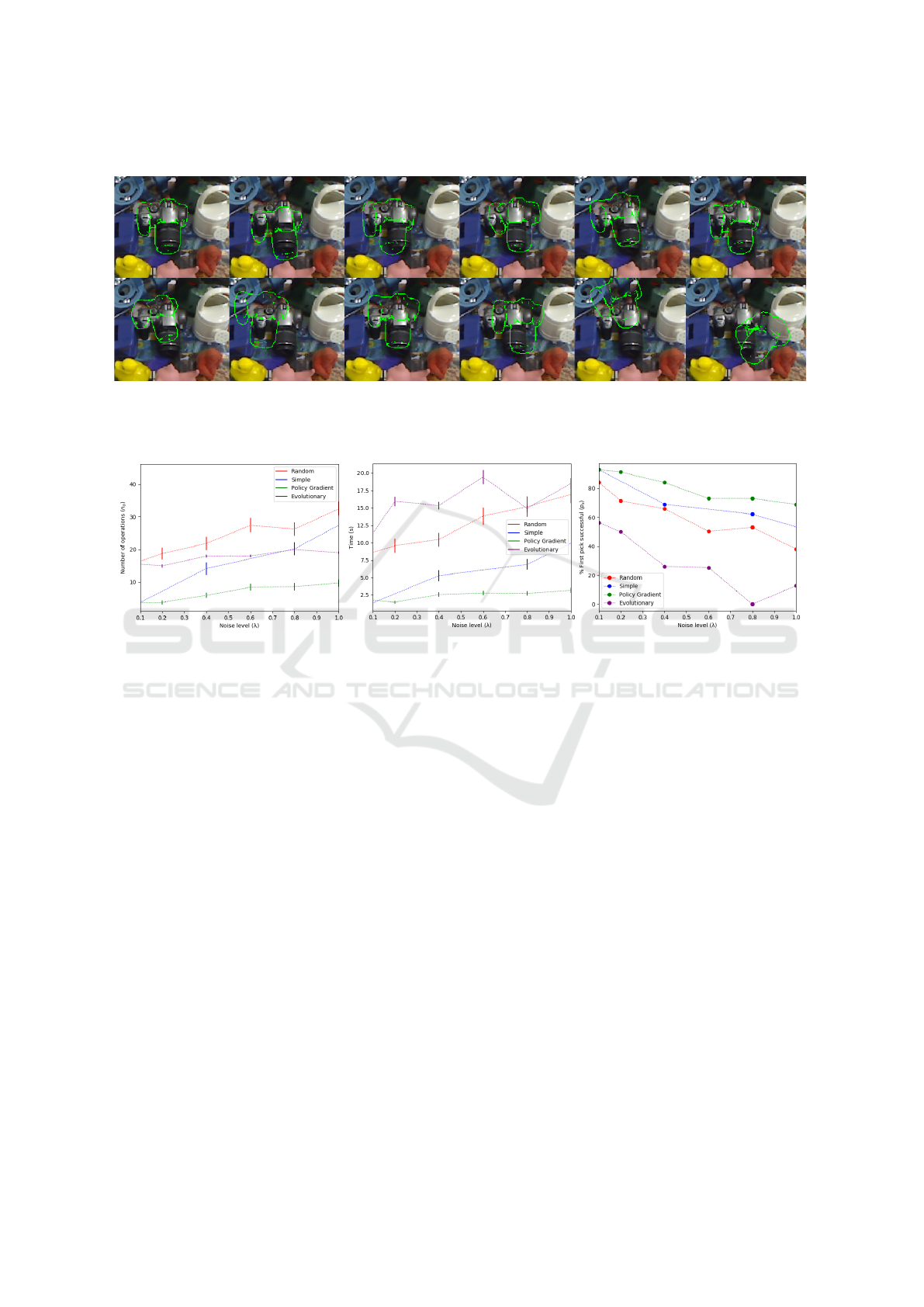
λ = 0.0 λ = 0.1 λ = 0.2 λ = 0.3 λ = 0.4 λ = 0.5

λ = 0.6 λ = 0.7 λ = 0.8 λ = 0.9 λ = 1.0 λ = 1.1

Figure 4: Examples of randomized noise levels from no noise (λ = 0.0) to noise level λ = 1.1 (as described in Sec. 5.1.1).

Noise is added on the 3-dimensional rotation and translation of the object position.

(a) Number of operations

(b) Time

Figure 5: Comparison of methods on the BOP LM dataset (see Sec. 5.2.1). Three types of metrics (see Sec. 6.2) were used

with noise levels λ ∈ {0.1, . . . , 1.0} (see Sec. 5.1.1).

iterations. This can be overcome be optimizing / par-

allelizing algorithmic components.

6.2.2 Computation Time

In Fig. 5b we evaluated the algorithms by the total

computation time required to reach a successful pick

averaged over all samples. The graph type is the same

as described in Sec. 6.2.1, where the quartile range for

each conﬁguration algorithm and λ noise value is in-

dicated by a vertical line. The evolutionary reinforce-

ment learning strategy shows the worst computational

performance, followed by the random agent. While

the simple agent shows a better performance over all

noise level, the best performing strategy in total time

until a successful pick per sample is the policy gra-

dient algorithm. Note, that the conﬁguration agent

takes the computation time into account, as the time

is returned as a negative reward component of the re-

ward created for each action. Future work will cover

the improvement of computation time through paral-

lelization as well as optimal data handling.

6.2.3 Successful First Picks

This metric evaluates how often a running algorithm

is correctly choosing the “pick” operator, when cho-

sen the ﬁrst time in the sequence. Consider our op-

erational elements: hypothesis generation (a

gen

) , hy-

pothesis reﬁnement (a

re f

) and pick operator (a

pick

). A

conﬁguration algorithm which chooses the following

sequence (0 indicating that the simulated pick failed

and 1 a successful pick operation):

gen

, a

re f

, a

pick

→ 0, a

re f

, a

pick

→ 1}

would arrive at a successful pick after 5 operations

(value 5 in “number of operations”, as shown in

Fig. 5a). In the metric of successful ﬁrst picks, it

would receive the value 0. Contrary, this sequence

would receive the value 1 (with value 5 in “number of

operations”):

gen

, a

re f

, a

re f

, a

re f

, a

pick

→ 1}.

We are expressing the results as percentage of suc-

cessful ﬁrst pick operations. The evaluation is shown

in Fig. 5c, where a higher value indicates a better

The Furtherance of Autonomous Engineering via Reinforcement Learning

performance. Note that, although the overall perfor-

mance of the evolutionary reinforcement algorithm is

superior to the random agent, it shows fewer success-

ful ﬁrst picks. This indicates, that a higher improve-

ment can be achieved by allowing for more agents

and iterations (which requires a compensation of the

run-time by parallelization). The simple agent shows

a better successful pick performance than the ran-

dom agent over all noise levels. The best performing

method in this metric is our policy gradient agent.

We evaluated the performance of all three metrics

additionally on our industrial dataset, which showed

comparable results in all categories.

7 CONCLUSIONS

Industrial production processes have a continuously

increasing need for ﬂexible and dynamic robotic so-

lutions. Today, this often requires long and tedious

conﬁgurations by well-trained engineers. Such pro-

cesses are both costly and time consuming. We target

this problem by learning optimized solutions, appli-

cable for a wide range of industrial tasks and environ-

ments. As an applicable precedent for such industrial

robotic engineering tasks, utilize the ﬁeld of robotic

picking.

We demonstrated our systematic approach of for-

mulating procedural knowledge in building blocks

and creating standardized interfaces. We evaluated

speciﬁc conﬁguration algorithms which were tasked

to choose such building blocks in an optimal order.

This was enabled by another standardized interface

for learning algorithms, namely the utilization of the

OpenAI Gym interface.

We showed, that an improvement of performance

with respect to a random or simple approach (as

could be performed by an engineered pipeline) can be

achieved for the task of 6D pose estimation for indus-

trial robotic picking for various scenarios (datasets).

From all evaluated conﬁguration algorithms, the pol-

icy gradient approach achieved the most superior per-

formance. We successfully demonstrated the gen-

eral feasibility of our approach on the public bop-

benchmark.

We demonstrated the setup and use of conﬁg-

uration algorithms and formally modeled building

blocks, both utilizing standardized interfaces (the

OpenAI Gym interface and a framework for hierar-

chical modeling respectively). This standardization

enables the dynamic connection of a wide range of

formally modeled building blocks and conﬁguration

algorithms. The more elements are available through

these frameworks, the more powerful our solution be-

comes. This will allow for a dynamic adaption to

a vast range of environments and objects with com-

plex shapes, surface reﬂection behaviors and textures.

Hence, one aspect of future work will lie in dimen-

sional scaling, such that our system holds numer-

ous elements (building blocks and conﬁguration al-

gorithms). Other aspects of future work will cover

the improvement of computational time of different

algorithmic components or the increase of computa-

tional power (e.g. by parallelization, using services

such as server clusters), enabling the evaluation of

a wider range of learning algorithms, as well as the

transfer of our algorithmic ideas to different areas of

industrial robotic applications.

ACKNOWLEDGEMENTS

This work was carried out within the Siemens AI Lab

Residency Program.

REFERENCES

Arun, K. S., Huang, T. S., and Blostein, S. D. (1987). Least-

squares ﬁtting of two 3-d point sets. IEEE Transac-

tions on Pattern Analysis and Machine Intelligence,

PAMI-9(5):698–700.

Brockman, G., Cheung, V., Pettersson, L., Schneider, J.,

Schulman, J., Tang, J., and Zaremba, W. (2016). Ope-

nai gym.

Chen, G., Han, K., Shi, B., Matsushita, Y., and Wong,

K.-Y. K. (2020). Deep photometric stereo for non-

lambertian surfaces.

Choi, C. and Christensen, H. I. (2016). Rgb-d object pose

estimation in unstructured environments. Robotics

Auton. Syst., 75:595–613.

Dietrich, V., Kast, B., Fiegert, M., Albrecht, S., and Beetz,

M. (2019). Automatic conﬁguration of the structure

and parameterization of perception pipelines. In 2019

19th International Conference on Advanced Robotics

(ICAR), pages 312–319.

El-Shamouty, M., Kleeberger, K., Laemmle, A., and Hu-

ber, M. (01 Nov. 2019). Simulation-driven machine

learning for robotics and automation. tm - Technis-

ches Messen, 86(11):673 – 684.

Hailin Jin, Soatto, S., and Yezzi, A. J. (2003). Multi-

view stereo beyond lambert. In 2003 IEEE Computer

Society Conference on Computer Vision and Pattern

Recognition, 2003. Proceedings., volume 1, pages I–

Hoda

n, T., Sundermeyer, M., Drost, B., Labb

e, Y., Brach-

mann, E., Michel, F., Rother, C., and Matas, J. (2020).

BOP challenge 2020 on 6D object localization. Euro-

pean Conference on Computer Vision Workshops (EC-

CVW).

ICINCO 2021 - 18th International Conference on Informatics in Control, Automation and Robotics

Hutter, F., Hoos, H. H., and Leyton-Brown, K. (2011). Se-

quential model-based optimization for general algo-

rithm conﬁguration. In Proceedings of the 5th Inter-

national Conference on Learning and Intelligent Op-

timization, LION’05, page 507–523, Berlin, Heidel-

berg. Springer-Verlag.

Hutter, F., Kotthoff, L., and Vanschoren, J., editors

(2018). Automated Machine Learning: Methods, Sys-

tems, Challenges. Springer. In press, available at

http://automl.org/book.

Imperoli, M. and Pretto, A. (2015). D

CO: Fast and robust

registration of 3D textureless objects using the Direc-

tional Chamfer Distance. In Proc. of 10th Interna-

tional Conference on Computer Vision Systems (ICVS

2015), pages 316–328.

Kast, B., Dietrich, V., Albrecht, S., Feiten, W., and Zhang, J.

(2019). A hierarchical planner based on set-theoretic

models: Towards automating the automation for au-

tonomous systems. In Gusikhin, O., Madani, K., and

Zaytoon, J., editors, Proceedings of the 16th Interna-

tional Conference on Informatics in Control, Automa-

tion and Robotics, ICINCO 2019 - Volume 1, Prague,

Czech Republic, July 29-31, 2019, pages 249–260.

SciTePress.

Kleeberger, K., Bormann, R., Kraus, W., and Huber, M. F.

(2020). A survey on learning-based robotic grasping.

In Current Robotics Reports, page pages239–249.

Koren, Y., Bell, R., and Volinsky, C. (2009). Matrix factor-

ization techniques for recommender systems. Com-

puter, 42(8):30–37.

Liu, M.-Y., Tuzel, O., Veeraraghavan, A., Taguchi, Y.,

Marks, T. K., and Chellappa, R. (2012). Fast ob-

ject localization and pose estimation in heavy clutter

for robotic bin picking. The International Journal of

Robotics Research, 31(8):951–973.

Lowe, D. G. (2004). Distinctive image features from

scale-invariant keypoints. Int. J. Comput. Vision,

60(2):91–110.

Rusinkiewicz, S. and Levoy, M. (2001). Efﬁcient variants

of the icp algorithm. In Proceedings Third Interna-

tional Conference on 3-D Digital Imaging and Mod-

eling, pages 145–152.

Song, K.-T., Wu, C.-H., and Jiang, S.-Y. (2017). Cad-based

pose estimation design for random bin picking using

a rgb-d camera. Journal of Intelligent and Robotic

Systems, 87.

Sun, M., Kumar, S., Bradsky, and Savarese, S. (2011). To-

ward automatic 3d generic object modeling from one

single image. In 3DIM-PVT.

Tang, J., Miller, S., Singh, A., and Abbeel, P. (2012). A tex-

tured object recognition pipeline for color and depth

image data. In ICRA, pages 3467–3474. IEEE.

Tekin, B., Sinha, S. N., and Fua, P. (2017). Real-time

seamless single shot 6d object pose prediction. CoRR,

abs/1711.08848.

Wanner, S. and Goldluecke, B. (2013). Reconstructing re-

ﬂective and transparent surfaces from epipolar plane

images. In Weickert, J., Hein, M., and Schiele, B.,

editors, Pattern Recognition, pages 1–10, Berlin, Hei-

delberg. Springer Berlin Heidelberg.

Yeh, T., Lee, J. J., and Darrell, T. (2009). Fast concur-

rent object localization and recognition. In 2009 IEEE

Conference on Computer Vision and Pattern Recogni-

tion, pages 280–287.

Zhou, Q.-Y., Park, J., and Koltun, V. (2018). Open3D:

A modern library for 3D data processing.

arXiv:1801.09847.

The Furtherance of Autonomous Engineering via Reinforcement Learning