Ground Speed Measuring System for Autonomous Vehicles
Yasmine Sheila Antille, Etienne Gubler and Juan-Mario Gruber
Institute of Embedded Systems, Zurich University of Applied Sciences, Winterthur, Switzerland
Keywords: Sensor Fusion, Ground Speed, Autonomous Driving, Driverless, Inertial Measurement Unit,
Global Positioning System, Kalman Filter.
Abstract: In this paper a Ground Speed Measuring System which can measure the ground speed over the ground in
three dimensions is proposed. The system uses two Kalman filters to compute the final ground speed based
on the readings from its various sensors. The proposed solution combines state of the art techniques from
different fields of sensor technology and will be incorporated into the high-performance driverless vehicle
after completion of this project. The findings and learnings of developing this system are discussed and an
evaluation of the module is presented. In the end, the system can accurately estimate a test vehicle’s ground
speed during system field tests.
1 INTRODUCTION
To be able to drive autonomously, a car depends on
precise sensor data and accurate algorithmic
calculations. Lots of various kinds of information is
required for autonomous driving. One of them is the
speed of movement of the vehicle over the ground.
To determine the ground speed of an autonomously
driving vehicle, multiple sensors can be fused
together to form a fail-safe system.
In this body of work we evaluate some of the
different possible approaches and then propose the
design and construction of a ground speed sensor
that measures the speed over the ground in 3
dimensions, and which can pass the data on to the
control unit of the vehicle. A prototype, focused on
economic efficiency, is developed and introduced
and the implementation is discussed. The algorithms
and system architecture are presented, which are
designed for robustness, reliability, and extensibility.
The ground speed measuring system is designed to
accurately measure and uses a set of measurements
generated by different sensors. The readings from
these sensors must be combined to determine an
estimate of the ground speed that is as accurate as
possible.
This work is carried out in cooperation with the
Formula Student ZHAW team and in close contact
with the driverless and electrical engineering teams.
2 GROUND SPEED SENSOR FOR
AUTONOMOUS VEHICLES
Driverless vehicles are autonomous cars in which
human drivers are never required to take control to
safely operate the vehicles. They combine sensors
and software to control, navigate, and drive the ve-
hicle without any human influence.
With a ground speed sensor and a suitable sensor
fusion algorithm, the vehicle’s odometry data will be
much more accurate than without such a system.
Having an accurate ground speed measurement can
therefore help refine the vehicle’s position while
mapping an environment. In addition, this will allow
for longer periods between the corrections the map-
ping algorithm has to undertake. With a Ground
Speed Measuring System (GSMS), it will also be
possible to recognize if one or more wheels lose
traction on the ground which could lead to an unfor-
tunate situation known as understeering. Like hu-
mans, autonomous vehicles could have difficulties
adapting quickly to loss of traction, therefore recog-
nizing such a situation as soon as possible can make
a huge difference in reaction time.
2.1 Formula Student
Formula Student is a worldwide competitive design
competition for student teams with the aim of build-
ing a race car. It provides a platform to student
Antille, Y., Gubler, E. and Gruber, J.
Ground Speed Measuring System for Autonomous Vehicles.
DOI: 10.5220/0010543106610668
In Proceedings of the 18th International Conference on Informatics in Control, Automation and Robotics (ICINCO 2021), pages 661-668
ISBN: 978-989-758-522-7
Copyright
c
 2021 by SCITEPRESS – Science and Technology Publications, Lda. All rights reserved
661

engineering teams for developing and enhancing
vehicle technologies in multiple domains. There are
three different competition categories: combustion
engine vehicles, electric vehicles and driverless
vehicles. The driverless category is the most recently
added one, having started in 2017. In the Formula
Student Driverless competition, a team is tasked to
build an autonomous race car that can complete the
racetracks without a driver’s influence by only using
onboard sensors and computers. The Formula Stu-
dent ZHAW team was formed by students from
different engineering backgrounds at the Zurich
University of Applied Sciences with the intention of
competing in the electric and driverless categories.
2.2 Related Work
Since 2017, hundreds of Formula Student teams
have been working on driverless vehicles. Outstand-
ing results and various publications have been deliv-
ered by the Academic Motorsports Club Zurich
(AMZ) from ETH Zurich.
In 2019, the AMZ-Racing driverless team pub-
lished a comprehensive report on the concept of
their first driverless racing car for the 2017/2018
racing season (Kabzan et al., 2017). The software-
hardware architecture of the developed “gotthard”
system is designed as follows. The software stack is
divided in three main modules: Perception, Motion
Estimation and Mapping and Control. Following the
architecture design, the velocity estimation is used to
compensate the motion distortion in the Lidar pipe-
line, propagate the state in the SLAM (Simultaneous
Localization and Mapping) algorithm, as well as
input for the control module. AMZ states in the
report that the velocity estimation needs to combine
data from various sensors with a vehicle model in
order for it to be robust against sensor failure and to
compensate for model mismatch and sensor inaccu-
racies. AMZ proposes to use a nine state Extended
Kalman Filter (EKF), which fuses data from six
different sensors.
AMZ also present the state estimation and sys-
tem integration for an autonomous race car in and
testify that sensor faults are a major factor under-
mining the robustness of state estimation systems
and, therefore, a probabilistic outlier detection
method should be used that works with any sensor.
Their approach makes use of the innovation covari-
ance calculated in the EKF which intrinsically ac-
counts for the uncertainty of the state and the sensor
noise model. Furthermore, they determine that if
wheel odometry is the only velocity source, and if
the wheels are constantly blocked due to high accel-
erations, the velocity estimate deteriorates (Valls et
al., 2018).
Of course, AMZ is not the only Formula Student
team that has achieved great results with a self-
developed measuring system that subsequently re-
sults in a ground speed estimation. To name a couple
of other remarkable approaches, two teams solved
this problem in the following ways:
The Viennese TUW Racing team uses a differen-
tial Global Positioning System (GPS), provided by a
Piksi Multi GNSS module along with two beacons
placed outside the racetrack. The beacons allow for
more precise positioning than a generic GPS system
does. To measure the relative movement of the vehi-
cle they included a motorsport-grade Inertial Meas-
urement Unit (IMU) (Zeilinger et al., 2017).
The Chinese BIT-FSD team relied mainly on
wheel speed sensors to calculate their first driverless
vehicle’s velocity in 2017. Even though their sensor
setup also includes GPS, INS, Lidar and camera
sensors, those are separately used to determine the
vehicle’s position and surroundings. Wheel speed
sensors are widely used for odometry calculations in
wheeled robots, where the team got this idea from
(Tian et al., 2018).
Generally, Bayesian filters provide a statistical
tool for dealing with measurement uncertainty,
which are described in an easy-to-follow way in
(Mochnac et al., 2009). This paper also explains that
the probability density function includes all infor-
mation needed to optimally solve estimation prob-
lems in a recursive way, which is why such filter
approaches are well suited for velocity estimation.
The Extended Kalman Filter is the state-of-the-art
estimator for fast, mildly non-linear systems and
provides a solution to this problem. The EKF works
by linearizing the involved models for every itera-
tion. The GSMS requires the use of an EKF for the
attitude estimation.
Noteworthy is also the Doppler-based approach
which a French research group from the Sorbonne
University Pierre and Marie Curie in Paris elaborate-
ly discuss in their paper (Lhomme-Desages et al.,
2009). With a low-cost Doppler radar and an accel-
erometer, the ground speed of a vehicle can also be
obtained. The focus of the paper lies on measuring
the slip rate, for which an estimation of the true
velocity of the vehicle with respect to the ground is
necessary. In this paper the authors do not resort to
wheel-based methods like optical encoders or re-
solvers. The Doppler effect principle is as follows: a
received electromagnetic wave’s frequency is com-
pared to a defined frequency, which changes as the
receiver moves with respect to the transmitter. For
ICINCO 2021 - 18th International Conference on Informatics in Control, Automation and Robotics
662

their sensor fusion, a simple Kalman filter suffices to
fuse the Doppler data and the accelerometer data
which outputs an estimate of the longitudinal veloci-
ty. With these calculations it is possible to measure
the slip rate for each wheel.
2.3 System Requirements
The general system requirement regarding a driver-
less race car is measurement certainty especially
while cornering and on wet subsoil. We posed the
following additional requirements for the developed
system regarding its expandability: The system can
be extended to allow further sensors to be added to
the sensor fusion without having to reorganise the
software structure. The system allows for a simula-
tion of recorded sensor data using tools such as
MATLAB. Additional redundancy checks can be
programmed to allow for even more precise system
outputs. The system can be fully integrated into the
future autonomous system of the Formula Student
ZHAW driverless car.
2.4 Sensor Placement
The sensors may be mounted to the vehicle with a
maximum distance of 500 mm above the ground and
less than 700 mm forward of the front tires as is
depicted in
Figure
1 . Furthermore, the vehicle is subjected to a
rain test at the races. Therefore, all sensors must be
adequately sealed and waterproof.
Figure 1: Envelope to mount sensor systems on a formula
student race car (FSG 2019).
3 SYSTEM CONCEPT AND
DESIGN
3.1 Overall Concept
The ground speed measuring system is designed to
accurately and reliably measure the ground speed of
an autonomous vehicle. The system features an
Inertial Measurement Unit (IMU) and Global Posi-
tioning Sensor (GPS) to measure the ground speed
as well as a microcontroller to process the raw sen-
sor readings.
3.2 Microcontroller and Sensors
With the sensor fusion of a GPS and an IMU the
GSMS can provide an accurate measurement output
which is based solely on the two sensors. The IMU
measures the following quantities:
• Acceleration (3D): X, Y and Z axes
• Angular velocity (3D): X, Y and Z axes
• Magnetic field strength (3D): X, Y and Z axes
The GPS measures the following quantities:
• Absolute position (3D): Latitude, Longitude,
Altitude
• Velocity (3D): Magnitude and angle relative to
(true) north, vertical velocity
3.3 Sensor Fusion and Data Processing
The measurements from the sensors are processed
and combined in a custom sensor fusion algorithm.
The custom sensor fusion algorithm consists of
multiple stages which perform different filtering and
fusion tasks. An overview of the different stages is
given in Figure 2. Readings from the implemented
sensors must be combined to determine an estimate
of the ground speed that is as accurate as possible,
for which the GSMS uses two Kalman filters as can
be seen in Figure 2. The first Kalman filter is only
used to determine the system attitude while the sec-
ond Kalman filter estimates the final system veloci-
ty.
Attitude Kalman Filter
The attitude Kalman filter is an EKF as the equa-
tions required to describe the physical properties of
the system attitude are non-linear. The attitude Kal-
man filter is used to track the system attitude, which
is represented using a quaternion (the first compo-
nent of the rotation quaternion describes the angle of
rotation and the remaining three components de-
scribe the axis of rotation). The attitude of the race
car is always described relative to the earth fixed
inertial reference frame.
The attitude Kalman filter has a state vector 𝑥
that tracks the x, y and z components of the attitude
error 𝑎 and the x, y and z components of the gyro-
scope bias. Therefore, the state vector is a column
vector with 6 elements. It is important to note that
the attitude Kalman filter does not directly track the
quaternion 𝑞

as part of its state vector. Instead, it
tracks an attitude error. At the beginning of each
iteration, this error is assumed to be zero.
Ground Speed Measuring System for Autonomous Vehicles
663

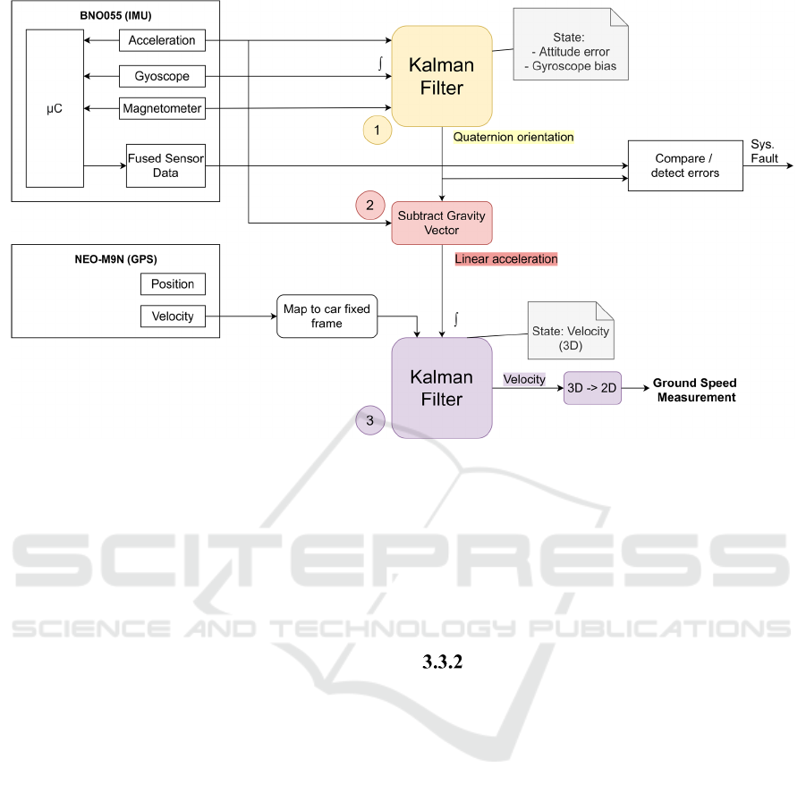
Figure 2: Sensor Fusion Concept.
And at the end of each iteration, the attitude er-
ror is added to the reference attitude quaternion
𝑞

and then reset to zero. The system attitude is
therefore expressed using two parts as described in
the following equation:
qt  δqat ⊕ 𝑞

t
(1)
The above approach of tracking an attitude error
instead of directly tracking the attitude is unique to
the attitude Kalman filter. The EKF used to track the
attitude in the GSMS therefore is a Multiplicative
Extended Kalman Filter (MEKF). The term "multi-
plicative" refers to the fact that the attitude error
𝑎𝑡 tracked by the attitude Kalman filter is propa-
gated to the reference attitude quaternion 𝑞

using
a quaternion multiplication operation. To perform
this quaternion multiplication at the end of each
iteration, 𝑎𝑡 is first converted into its quaternion
representation and then multiplied with 𝑞

.
Instead of changing the attitude error 𝑎𝑡, the
prediction step directly adjusts the reference quater-
nion 𝑞

. After 𝑞

has been updated, the error
covariance matrix 𝑃 must be updated as well. This is
required as the process model introduces new errors.
These errors are represented by the process noise
covariance matrix 𝑄. The steps to update 𝑃 therefore
involve the matrix 𝑄. The measurement step of the
attitude Kalman filter corrects the previously calcu-
lated estimate using absolute measurements of the
system attitude. The measurement step is executed
twice, as the GSMS uses the gravity vector given by
the accelerometer and the North vector given by the
magnetometer as two absolute measurements for the
system attitude. Finally, the error propagation step
must always be called before a new iteration of the
attitude Kalman filter algorithm is started.
Velocity Kalman Filter
The velocity Kalman filter is a regular Kalman filter
as the equations required to describe the system
velocity are all linear. This makes the velocity Kal-
man filter significantly simpler than the attitude
Kalman filter. The velocity Kalman filter can also
directly track the velocity of the system in its state
vector 𝑥. The state vector 𝑥 for the velocity Kalman
filter contains the x, y and z components of the sys-
tem velocity.
The initial value for the state vector 𝑥 is set to
the zero vector. The state vector directly tracks the
system velocity. Setting the state vector 𝑥 to the zero
vector therefore results in the following initial condi-
tion: The system velocity 𝑣𝑒𝑙 is set to the zero vec-
tor. The system is usually initialized while the race
car is not moving, therefore the above initial value
for the system velocity 𝑣𝑒𝑙 is a reasonable choice.
The velocity Kalman filter predicts the system
velocity by integrating the linear acceleration meas-
ured using the accelerometer. The integral over the
linear acceleration 𝑙𝑖𝑛_𝑎𝑐𝑐𝑒𝑙 is computed using the
ICINCO 2021 - 18th International Conference on Informatics in Control, Automation and Robotics
664

time 𝑑𝑡 that has passed since the last iteration of the
algorithm. The GSMS is designed such that 𝑑𝑡 is
always 10ms. After the state vector 𝑥 has been up-
dated, as for the MEKF, the error covariance matrix
𝑃 must be updated as well. These errors are repre-
sented by the process noise covariance matrix 𝑄.
The measurement step of the velocity Kalman
filter will correct the previously calculated estimate
using an absolute measurement of the system veloci-
ty. The GSMS uses the velocity measured in 3 di-
mensions by the GPS as absolute measurements for
the system velocity.
4 RESULTS
To test the developed system, we made the follow-
ing comparisons:
• The output of the custom attitude Kalman filter
algorithm was compared to the output of the
sensor fusion firmware, which runs on the
IMU.
• The output of the custom velocity Kalman fil-
ter algorithm was compared to the GPS veloci-
ty measurement (which is only available at a
lower frequency than the output of the velocity
Kalman filter).
4.1 Attitude Kalman Filter
The first test was carried out in a residential area by
driving around two blocks in a figure of 8. This test
was performed at low speeds of around 30 km/h. The
goal of this test was to demonstrate that the algo-
rithms of the GSMS are processing the sensor data
correctly. The accuracy is only evaluated in a qualita-
tive manner. The performance of the attitude Kalman
filter is demonstrated very well using this test. Driv-
ing a figure of 8 involved turns in both directions and
it ensured that the vehicle was oriented in a variety of
different directions throughout the test.
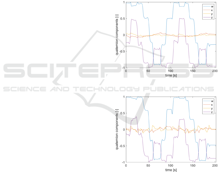
The attitude is represented as a rotation consist-
ing of four components. All attitude plots display the
w, x, y and z components of the quaternion separate-
ly. Due to the trigonometric functions involved in
the quaternion representation of a rotation, the
meaning of individual components of a quaternion is
often difficult to interpret. Certain individual com-
ponents displayed in the attitude plots manage to
show specific properties of the tests, which will be
explained for each plot.
Figure 3 clearly demonstrates that our custom at-
titude Kalman filter calculates a meaningful system
attitude. This claim is supported by the following
observations: The graph shows that the x and y
components of the plot remain roughly constant
around zero. This is the expected behaviour if the
vehicle is only rotated around its z axis. The graph
also shows that the z component of the quaternion
continuously changes its value throughout the test.
This is the expected behaviour if the vehicle is driv-
ing a figure of 8 on a horizontal plane.
The attitude computed by the custom sensor fu-
sion algorithm can now be compared to the attitude,
that is computed by the bno055 sensor fusion firm-
ware. The output of the sensor fusion firmware is
displayed in Figure 4.
Figure 3: System Attitude (as computed by the custom
attitude Kalman filter).
Figure 4: Actual system attitude (as computed by the
bno055 firmware).
This graph allows us to prove that the GSMS
does not only calculate a meaningful system attitude,
but that it is also in line with the output of an inde-
pendent algorithm. When comparing the two graphs
the following can be observed: The custom sensor
fusion algorithm implemented in the GSMS com-
Ground Speed Measuring System for Autonomous Vehicles
665

putes (qualitatively) the same attitude as the bno055
sensor fusion firmware. The custom sensor fusion
algorithm correctly processes the input of all three
sensors (accelerometer, gyroscope and magnetome-
ter). The x and y axis of the attitude quaternion
measured by our custom sensor fusion algorithm
shows higher fluctuation than the output computed
by the bno055 sensor fusion firmware. The reason
for this is unknown.
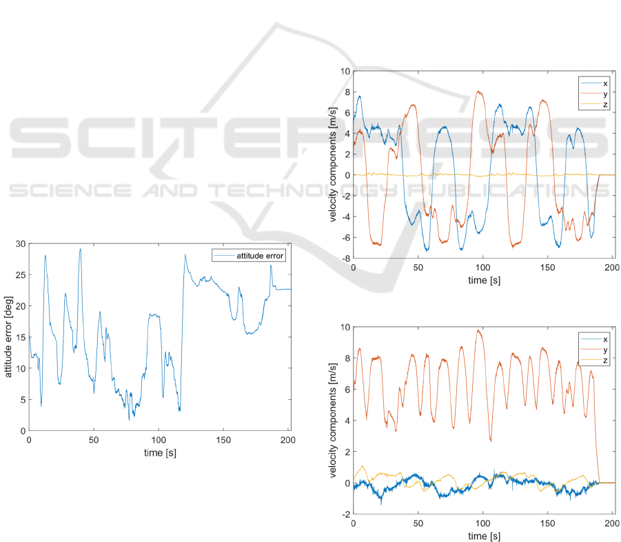
Figure 5 shows the angle of the difference in ro-
tation between the attitude computed by the GSMS
and by the bno055 sensor fusion firmware. This plot
effectively visualizes the difference between the two
plots shown before. The plot shows that the differ-
ence between the two attitude measurements is usu-
ally between 5 and 25 degrees. Our experiments
showed that this is mostly caused by magnetic dis-
turbances which influence the measurement made by
the magnetometer inside the IMU. The custom sen-
sor fusion firmware starts to output inaccurate atti-
tude values if the magnetometer is not in an ideal
environment.
The bno055 sensor fusion firmware on the other
hand seems to have a mechanism that detects situa-
tions where magnetometer measurements are unreli-
able. It then most likely stops relying on the magne-
tometer input until it is able to re-calibrate the mag-
netometer. The strong magnetic disturbances were
mostly caused by the residential area in which this
test was performed. The second test was performed
in an area with less buildings which lead to an im-
proved performance of the custom attitude Kalman
filter.
Figure 5: Attitude error.
4.2 Velocity Kalman Filter
The test described above is also well suited to
demonstrate the performance of the velocity Kalman
filter. Figure 6 shows the velocity as it was recorded
by the GPS. The plot visualizes all three axes which
correspond to the 𝑁𝑜𝑟𝑡ℎ

𝑥

,𝐸𝑎𝑠𝑡𝑦 and 𝑈𝑝𝑧
axes of the inertial frame. It is important to note that
the following plot shows the GPS measurement,
which is always made in the inertial frame. The plot
shows that the car was moving in different directions
on a horizontal plane. Therefore, the GPS measured
non-zero values on the x and y axis while the z axis
remained constant at zero velocity. This is the ex-
pected behaviour.
The plot in Figure 7 shows how the previously
calculated system attitude is used to transform the
GPS velocity from the inertial frame into the body
frame. This plot displays the same velocity as Figure
6 but after it was rotated into the body frame using
the system attitude computed by the GSMS. Thus,
the plot now shows the three axes x, y and z corre-
sponding to the body frame. We can clearly see that
the plot only shows a significant velocity for the y
axis. This is the expected behaviour because the y
axis is facing in the direction of travel. This is fur
Figure 6: GPS velocity.
Figure 7: Rotated GPS velocity.
ICINCO 2021 - 18th International Conference on Informatics in Control, Automation and Robotics
666

ther proof that the attitude Kalman filter is in fact
computing the correct attitude. Because the trans-
formation from Figure 6 to Figure 7 is solely based
on this attitude. An incorrect attitude would have
caused high non-zero values on the x and z compo-
nents in Figure 7.
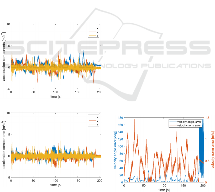
4.3 Linear Acceleration
Figure 8 displays the linear acceleration calculated
by the GSMS after the gravity vector has been sub-
tracted. Subtracting the gravity vector again involves
the previously calculated system attitude.
Figure 9 displays the linear acceleration as it was
calculated by the bno055 sensor fusion firmware.
These two plots show a similar linear acceleration.
Especially high peaks of acceleration are found in
both plots. The plots do however not meet the ex-
pected behaviour. The expected behaviour would be
that both plots continuously show the same values
on all three axes. We expect some interference to
cause this unexpected behaviour.
Figure 8: Kalman filter linear acceleration.
Figure 9: Actual linear acceleration.
4.4 Final System Output
This part of the test compares the final output of the
custom velocity Kalman filter implemented in the
GSMS with the rotated velocity measurement that
was recorded by the GPS. Figure 10 visualizes the
error between the velocity Kalman filter output and
the rotated GPS velocity.
The plot shows two different properties: The an-
gle between the two velocity vectors in degrees
(velocity angle error) and the difference in length
between the two velocity vectors in m/s (velocity
norm error).
The graph can be interpreted as follows: The ve-
locity angle error is usually below 20 degrees and
often below 10 degrees. This is the expected behav-
iour. It proves that the direction of the velocity
measured by the GSMS is correct. The velocity
norm error is usually below 1 m/s. This is the ex-
pected behaviour. It proves that the absolute value of
the velocity measured by the GSMS is correct. The
velocity angle error increases to values of up to 180
degrees at the very end of the test. This is the ex-
pected behaviour for situations where the actual
velocity is zero. At the very end of the test, the vehi-
cle was stationary after coming to a halt, and there-
fore the GSMS as well as the GPS are measuring
velocity vectors which are very close to the zero
vector. It is expected that the angle between those
two vectors can assume any angle in the range of 0
to 180 degrees, as seen in the graph.
Figure 13 shows the final output of the GSMS.
This is the signal which will be transmitted to the
control unit of the self-driving car. It shows the three
components of the vehicle ground speed in the body
frame. It clearly shows that the main part of the
velocity is measured on the y axis which is facing in
the direction of travel. This is the expected behav-
iour.
Figure 10: Velocity error.
Ground Speed Measuring System for Autonomous Vehicles
667

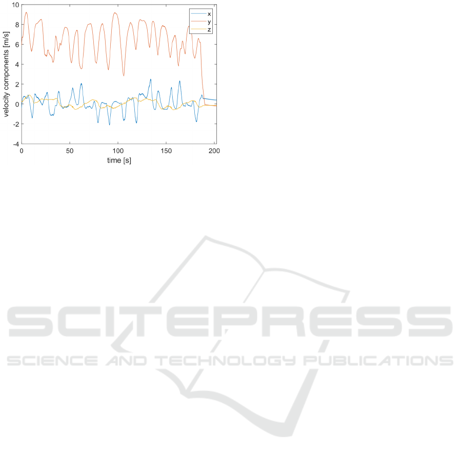
Figure 11: Kalman filter velocity output.
5 CONCLUSIONS
One of the main motivations for developing a
ground speed measuring system was to take part in
the development of an autonomous race car. The
idea was to have a reliable and redundant measuring
system support the driverless vehicle in various
aspects with this sensor fusion output, in order to be
eligible to compete with top teams around the world.
In this paper, an approach to a ground speed
measuring system using two sensors providing data
for sensor fusion was presented. Details were pro-
vided on the hardware and software architecture.
The presented ground speed measuring system
proved its functionality during testing. The tests
performed on the GSMS showed that the custom
sensor fusion algorithms are mathematically correct.
They produced a qualitatively acceptable and usable
output in all tests.
However, the sensor fusion algorithms start to
produce inaccurate outputs if the environment does
not provide ideal conditions. This could be improved
by adding more features to the currently implement-
ed algorithms of the GSMS, such as detection of
incorrect sensor measurements (especially for the
magnetometer) and/or additional filtering of sensor
measurements prior to executing the Kalman filters
(specifically a high pass filter for the gyroscope and
a low pass filter for the accelerometer when deter-
mining the gravity vector).
REFERENCES
Kabzan, J. et al. (2017). Autonomous Racing Car for
Formula Student Driverless. ROSCon Vancouver 2017.
doi:10.36288/roscon2017-900803
Valls, M. I. et al. (2018). Design of an Autonomous Race-
car: Perception, State Estimation and System Integra-
tion. 2018 IEEE International Conference on Robotics
and Automation (ICRA). doi:10.1109/icra.2018.
8462829
Zeilinger, M. et al. (2017). Design of an Autonomous
Race Car for the Formula Student Driverless (FSD).
Proceedings of the OAGM&ARW Joint Workshop
2017. doi: 10.3217/978-3-85125-524-9-10
Tian, H., Ni, J., & Hu, J. (2018). Autonomous Driving
System Design for Formula Student Driverless Race-
car. 2018 IEEE Intelligent Vehicles Symposium (IV).
doi:10.1109/ivs.2018.8500471
Mochnac, J., Marchevsky, S., & Kocan, P. (2009). Bayes-
ian filtering techniques: Kalman and extended Kalman
filter basics. 2009 19th International Conference Ra-
dioelektronika. doi:10.1109/radioelek.2009.5158765
Lhomme-Desages, D., Grand, C., Guinot, J., & Amar, F. B.
(2009). Doppler-Based Ground Speed Sensor Fusion
and Slip Control for a Wheeled Rover. IEEE/ASME
Transactions on Mechatronics, 14(4),484-492.
doi:10.1109/tmech.2009.2013713
FSG (2019, September 13). Formula Student
Rules 2020. Retrieved February 10, 2021, from
https://www.formulastudent.de/fileadmin/user_upload/
all/2020/rules/FS-Rules_2020_V1.0.pdf
ICINCO 2021 - 18th International Conference on Informatics in Control, Automation and Robotics
668