Task-motion Planning via Tree-based Q-learning Approach for Robotic
Object Displacement in Cluttered Spaces
Giacomo Golluccio, Daniele Di Vito, Alessandro Marino, Alessandro Bria and Gianluca Antonelli
∗
Department of Electrical and Information Engineering,
University of Cassino and Southern Lazio, via Di Biasio 43, 03043 Cassino (FR), Italy
Keywords:
Motion Planning, Task Planning, Reinforcement Learning.
Abstract:
In this paper, a Reinforcement Learning approach to the problem of grasping a target object from clutter by
a robotic arm is addressed. A layered architecture is devised to the scope. The bottom layer is in charge of
planning robot motion in order to relocate objects while taking into account robot constraints, whereas the top
layer takes decision about which obstacles to relocate. In order to generate an optimal sequence of obstacles
according to some metrics, a tree is dynamically built where nodes represent sequences of relocated objects and
edge weights are updated according to a Q-learning-inspired algorithm. Four different exploration strategies
of the solution tree are considered, ranging from a random strategy to a ε-Greedy learning-based exploration.
The four strategies are compared based on some predefined metrics and in scenarios with different complexity.
The learning-based approaches are able to provide optimal relocation sequences despite the high dimensional
search space, with the ε-Greedy strategy showing better performance, especially in complex scenarios.
1 INTRODUCTION
Nowadays, the problem of retrieving objects from
clutter is of particular interest in fields like industrial
and assistive robotics. This involves the robot plan-
ning over a task-motion space, and combining dis-
crete decisions about objects and actions with con-
tinuous decisions about collision-free paths (Dantam
et al., 2016). A vast portion of industrial processes
are characterized by a static environment with known
object positions, and thus can be easily automated ex-
ploiting the advances in robot technologies such as
mechanism design and control (Lee et al., 2019).
On the other hand, grasping a target from clut-
ter in assistive scenarios remains challenging due to
a highly unstructured environment populated by a
variety of objects arranged irregularly and accessi-
ble only after relocating other objects (Cheong et al.,
2020). Since isolated motion planning typically as-
sumes a fixed configuration space, integrated Task-
Motion Planning (TMP) that orchestrates high level
task planning and low-level motion planning is re-
quired in this scenario. Moreover, the problem of
∗
This work was supported by the Dipartimento di Ec-
cellenza through the Department of Electrical and Informa-
tion Engineering (DIEI), University of Cassino and South-
ern Lazio
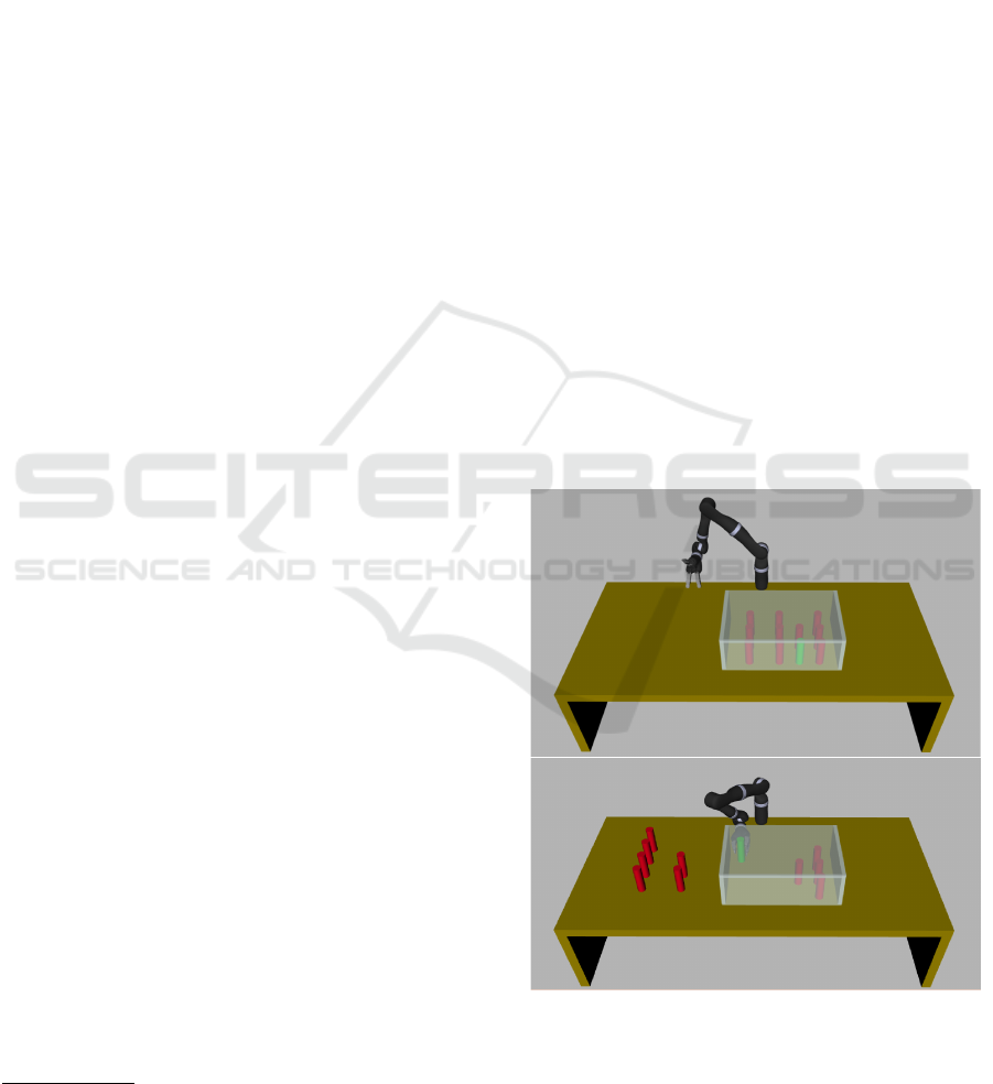
Figure 1: An example of cluttered environment. The target
is represented by the cylinder in green, while obstacles are
in red. Starting from the scenario on the top, the manipula-
tor is required to relocate some obstacles in order to grasp
the target (bottom scenario).
planning for object rearrangement has been shown to
be N P -hard (Cheong et al., 2020).
130
Golluccio, G., Di Vito, D., Marino, A., Bria, A. and Antonelli, G.
Task-motion Planning via Tree-based Q-learning Approach for Robotic Object Displacement in Cluttered Spaces.
DOI: 10.5220/0010542601300137
In Proceedings of the 18th International Conference on Informatics in Control, Automation and Robotics (ICINCO 2021), pages 130-137
ISBN: 978-989-758-522-7
Copyright
c
 2021 by SCITEPRESS – Science and Technology Publications, Lda. All rights reserved

A number of approaches have been proposed in
literature to overcome the abovementioned issues.
In (Dogar et al., 2014) it is reported an algorithm that
computes a sequence of objects to be removed while
minimizing the expected time to find a hidden target.
This presents difficulties linked to running time, con-
sequently in a very cluttered environment it might be
inoperable. A similar problem is solved in (Srivastava
et al., 2014), but the minimization of the number of
actions is neglected, while in (Lagriffoul et al., 2014),
a combined task and motion planning with the aim to
reduce the dimensionality of search space through a
constraint-based approach is proposed. In (Nam et al.,
2020), the Authors compute the object to relocate by
building a traversability graph in a static and known
environment with a heuristics in the order to grasp the
objects based on their volumes.
An interesting area of machine learning is Rein-
forcement Learning (RL) that concerns an agent pro-
ceeding by trial-and-error in a complex environment
in order to maximize a cumulative reward that ul-
timately leads to the goal achievement. Recently,
RL techniques have received a growing share of re-
search in the field of combined TMP (Eppe et al.,
2019) including object manipulation and grasping in
a cluttered environment (Mohammed et al., 2020). In
this context, a widely used approach is to train an
end-to-end deep-RL model that takes a visual input
(e.g. single- or multi-view RGB or RGB-D image)
and maps it to feasible actions that lead to the goal
(Deng et al., 2019; Yuan et al., 2019). This is pos-
sible by leveraging the recent advances in deep con-
volutional neural networks (LeCun et al., 2015) and
value/policy-based RL (Mnih et al., 2013). Despite its
merits, deep-RL-based robotic grasping might have
some limitations such as the difficulty to interpret
the deep neural network model, the high computa-
tional complexity and the requirement of a significant
amount of attempts, before to reach convergence.
In this paper, we propose a method to solve pick-
and-place problems in a cluttered environment inte-
grating TMP and Q-value-based RL. The idea is to
find the optimal sequence of obstacles to relocate us-
ing Q-learning (Watkins and Dayan, 1992; Jang et al.,
2019) in order to reach the target taking into account
kinematic constraints. The innovative contribution is
twofold: firstly, we design an ordered-tree structure
(Q-Tree) that replaces the traditional value-matrix in
Q-learning, and adapt the learning algorithm accord-
ingly; secondly, we integrate in the Q-Tree learning
the motion planner based on the inverse kinematics
framework proposed in (Di Vito et al., 2020).
2 PROBLEM FORMULATION
AND MATHEMATICAL
BACKGROUND
2.1 Problem Formulation
In this paper, we consider the problem of moving a
target object T from its initial location p
t,0
∈ IR
3
to a
final one p
t, f
∈ IR
3
from clutter; therefore, in order to
achieve this objective, it might be required to relocate
some of or all the N
o
obstacles O = {O
1
,... ,O
No
}
present in the scene having position p
o,i
∈ IR
3
(i =
1,2, ·· · ,N
o
). Furthermore, target grasping and ob-
ject relocation are performed by a robot manipulator;
an illustrative scenario is reported in Figure 1, where
the initial scene is shown in the top image, while the
scene after obstacles relocation is shown in the bot-
tom.
An object, either a target or an obstacle, is occluded if
no trajectory for the robot exists to grasp and relocate
it, that means that other objects prevent the robot end
effector from reaching the object.
Let us denote with H the initial configuration of
the scenario, where the robot is in its home posi-
tion and neither obstacles nor the target were relo-
cated, with S
k
= {O
i
1
, ·· · , O
i
k
} any sequence of car-
dinality |S
k
| = k and with S
T
k
the sequence {S
k−1
, T },
i.e. the sequence obtained from S
k−1
by adding T
as last element. In particular, the generic object O
i
j
( j = 1,.. ., k) inside a sequence S
k
is defined relocat-
able if all precedent ones {O
i
1
, ·· · , O
i
j−1
} can be re-
located. Thus, a sequence S
k
(or S
T
k
) is considered
feasible if all its objects are relocatable. Since multi-
ple feasible sequences generally exist, an optimal (or
sub-optimal) sequence should be searched for. In this
case, for example, the cardinality of the sequence is
considered. The following assumptions are made.
Assumption 1. The scene configuration in terms of
target location and obstacles positions is known be-
forehand.
Assumption 2. Objects are relocated without affect-
ing the remaining ones.
Assumption 3. For both obstacles and target, only
side grasp is allowed.
In this paper, Reinforcement Learning is adopted
as a tool to learn an optimal (or sub-optimal) feasible
sequence on a tree data structure, for which basics are
reported in the following.
Task-motion Planning via Tree-based Q-learning Approach for Robotic Object Displacement in Cluttered Spaces
131

2.2 Reinforcement Learning
The Reinforcement Learning approach is, in general,
a trial-and-error based technique, i.e., an agent iter-
atively makes observations and takes actions within
an environment while receiving feedback referred to
as reward. In detail, at each time step k and given a
state s
k
, the agent selects an action a
k
and receives a
scalar reward r
k
, trying to maximise the expected re-
ward over time. More in detail, the decision-making
problem is modelled as a Markov decision process
(MDP), that is defined as a tuple (S ,A, p,r,γ) where S
is the state space, A is the action space, p = Pr(s
k+1
=
s
0
|s
k
= s, a
k
= a) is the transition probability from the
current state to the next one, r is the reward function
and γ ∈ [0,1] is the discount factor tuning the rewards
weight on the agent action selection. factor, γ ∈ [0,1]
In order to decide what action to take at a particu-
lar time step, the agent has to know how good a par-
ticular state is. A way of measuring the state good-
ness is the action-value function also known as the
Q-function, defined as the expected sum of rewards
taking action a
k
in the state s
k
following a policy π:
Q
π
(s,a) = E
π
(
∞
∑
l=0
γ
l
r
k+l+1
|s
k
= s,a
k
= a) . (1)
Since the agent aim is to maximise the expected
cumulative reward, the optimal action-value function
is given by
Q
∗
(s,a) = max
π
Q
π
(s,a), ∀s ∈ S,a ∈ A , (2)
which combined with the Eq. (1) leads to the Bellman
optimality equation
Q
∗
(s,a) =
∑
s
0
p(s
0
|s,a)[r
k+1
+ γmax
a
0
Q
∗
(s
0
,a
0
)] , (3)
where s
k
= s, s
k+1
= s
0
,a
k
= a, a
k+1
= a
0
, respectively.
Equation (3) takes into account the state transition
probability p(s
0
|s,a) which assumes the knowledge
of the environment model, i.e., a model-based prob-
lem. However, the same expression can be adopted
for model-free approaches as well. In the latter case,
the state transition probability is set to one resulting
in the following:
Q
∗
(s,a) = r
k+1
+ γmax
a
0
Q
∗
(s
0
,a
0
) . (4)
How it is noticeable, the expression in Eq. (4) is a
recursive nonlinear function with no closed form so-
lution. For this reason, several iterative approaches
have been proposed in literature like Q-learning
in (Watkins and Dayan, 1992). According to this ap-
proach, the following iterative update law is adopted:
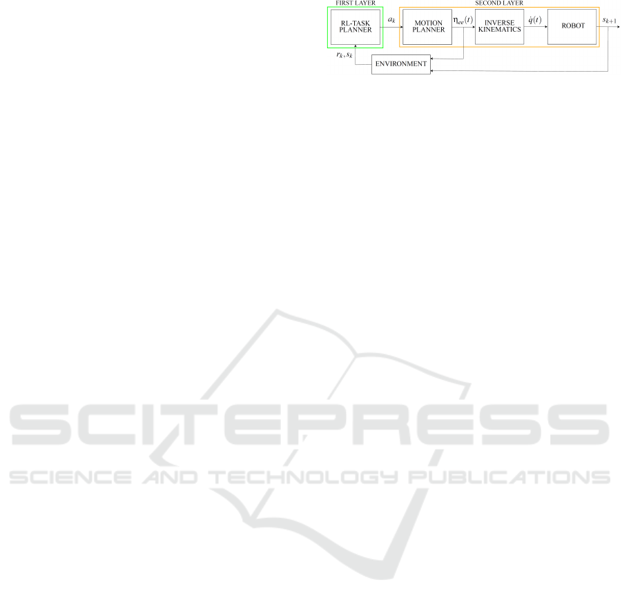
Figure 2: The proposed architecture. The RL-Task Planner
choices the action a
k
with an appropriate policy, while the
Motion Planner provides the feasibility of request. The In-
verse Kinematics block sends the reference signal to Robot
that acts the motion. The environment elaborates feedback
signals from Motion Planner and Robot updating the agent.
Q
k+1
(s
k
,a
k
) =Q
k
(s
k
,a
k
) + α(r
k+1
+
γmax
a∈A
Q
k
(s
k+1
,a) − Q
k
(s
k
,a
k
)) .
(5)
where α ∈ [0,1] is a hyper-parameter known as learn-
ing rate.
3 PROPOSED SOLUTION
Aimed at solving the problem described in Sect. 2.1,
we propose the architecture in Figure 2 that is a two-
layer architecture, where the high level (the RL-Task
Planner block) is in charge of learning the optimal
(according to a predefined metrics) feasible sequence
of obstacles to relocate in order to reach and grasp
the target, while the low level (the Motion planner,
Inverse kinematics (IK) and Robot blocks) is in charge
of providing information to the former about feasility
of robot movement.
It is worth noticing that the word Task used within
the low level context does not refer to the high level
discrete planning, unlike all the other sections of this
work. Indeed, regarding the constrained planning de-
scribed in next Section, it concerns analytical func-
tions representing control objectives inside the inverse
kinematics framework.
3.1 Constrained Planning
As mentioned before, the motion planner is in charge
of planning feasible trajectories η
ee
(t) for the robotic
manipulator end-effector to grasp and relocate ob-
jects (either the target or an obstacle) in the scene
as selected by the task planning layer. In partic-
ular, it is designed as two processes that are the
sampling-based algorithm and the Set-based Task-
Priority Inverse Kinematics (STPIK) check, respec-
tively (Di Vito et al., 2020). The sampling-based al-
gorithm is performed for planning a feasible trajec-
tory only in the Cartesian space. Thus, the sampling-
related computational load is kept down. All the con-
straints in the system joint space are then verified in
ICINCO 2021 - 18th International Conference on Informatics in Control, Automation and Robotics
132

the second process, i.e., the STPIK-check. The lat-
ter process consists of verifying the output trajectory
η
ee
(t) feasibility through the Set-based Task-Priority
Inverse Kinematics framework. This framework is
used for the local controller as well. Thus, in case
of static environment the trajectory tracking by the
robotic system is guaranteed.
Given a robotic manipulator system with n DOFs
and, therefore, q = [q
1
.. .q
n
]
T
its joint space, the
STPIK framework allows to performs several priority
ordered tasks simultaneously in addition to the end-
effector pose η
ee
, such as, e.g., obstacle avoidance,
virtual walls and joint limits. In particular, the i-th
task σ
i
can be set in a priority hierarchy H such that
the velocity components of the lower priority task are
projected into the null space of the higher priority
one. In this way, the highest priority task is always
guaranteed. Thus, given h tasks, the joint velocities ˙q
are computed as (Siciliano and Slotine, 1991)
˙q
h
=
h
∑
i=1
(J
i
N
A
i−1
)
†
(
˙
σ
i,d
+ K
i
˜
σ
i
− J
i
˙q
i−1
) , (6)
where N
A
i
is the null space of the augmented Jacobian
matrix J
A
i
stacking the task Jacobian matrices from
task 1 to i,
˙
σ
d
is the time derivative of the task desired
value σ
d
, K is a positive-definite gain matrix and
˜
σ =
σ
d
− σ is the task error.
Equation 6 allows to implement the Task-Priority
Inverse Kinematics (TPIK) for running multiple tasks
simultaneously. The latter are equality-based tasks,
i.e., they present a specific desired value as control
objective. However, tasks such as joint limits and ob-
stacle avoidance, present a set of allowed values and,
therefore, they are defined as set-based tasks. Within
the aim to manage this kind of tasks as well, the
Set-based Task-Priority Inverse Kinematics (STPIK)
algorithm, first proposed in (Di Lillo et al., 2020)
and (Di Lillo et al., 2021), is here exploited. The
key idea of this method consists of considering the
generic set-based task σ as disabled, i.e., not included
in the hierarchy, until it is in the valid range of val-
ues σ
a,l
< σ < σ
a,u
, and enabled, i.e., included in the
hierarchy as a high priority equality task, when it ex-
ceeds a predefined lower σ
a,l
or higher σ
a,u
activa-
tion threshold. In this way both equality and set-based
tasks are properly considered.
3.2 RL-Task Planner
Given N
o
obstacles, the number of possible sequences
S made of k ≤ N
o
obstacles with the target T as last
Figure 3: An example of complete Q-Tree. The node root
s
H
represents the initial configuration where all objects are
in the initial location. The last nodes s
N
0
+1,T
represent the
states that contain the target.
element of the sequence is
ξ
t
=
No
∑
i=1
i!

N
o
i

, (7)
which is obtained by considering all permutations
without repetition of k obstacles and where the order
matters, plus the target as last element. Obviously, not
all these sequences are feasible in the sense defined in
Sect. 2.1 and, as already mentioned, we are interested
in efficiently exploring the search space so as to find,
among the feasible solutions, optimal ones according
to a given metrics. The proposed method, named Q-
Tree significantly limits the computational burden.
According to the RL formulation (see Sect. 2.2),
actions and reward function need to be defined for
the problem at hand. The set of actions A =
{a
1
, ·· · ,a
N
o
, a
T
} is such that a
i
(i = 1, 2,· ·· , N
o
) and
a
T
represent the request to the motion planner layer
(see Figure 2) to relocate obstacle O
i
and target T,
respectively.
Therefore, given an action in the set A, the motion
planner layer provides a binary feedback to the task
planning layer regarding the possibility to relocate an
object, while meeting all kinematic constraints. In
case an object is relocatable.
With regards to the reward function r introduced
in Sect. 2.2, the following expression is adopted
r(s, a) =





0, if grasp
O
−1, if grasp
100, if grasp
T
, (8)
meaning that, given a state s ∈ S and an action a ∈ A,
the reward is:
Task-motion Planning via Tree-based Q-learning Approach for Robotic Object Displacement in Cluttered Spaces
133

• 0 if the obstacle i can be relocated according to
the feedback provided by the motion planner;
• −1 if either an obstacle or the target cannot be
relocated because of occlusions and robot con-
straints;
• 100 if a = a
T
and the target can be grasped and
relocated.
Based on this information, the weighted directed tree
structure is dynamically updated. In details, a se-
quence S
s
k
is associated to each node s
k
of the tree and
corresponds to the objects that have been relocated so
far (the sequence might be either feasible or unfea-
sible); the sequence S
s
H
associated to the root node,
s
H
, corresponds to the state in which no object was
relocated and is the empty sequence (i.e., S
s
H
= {}).
Starting from a given node s
k
, the next action from the
set A corresponding to those objects that have not yet
been relocated, and that the motion planner has not
already tried to relocate without success is selected;
then, two cases are possible: (i) if an action is se-
lected for the very first time from the current node, a
new child node s
k+1
is generated with associated se-
quence S
k+1
= {S
k
,O
i
} or S
T
k
= {S
k
,T } depending on
selected action (a
i
or a
T
, respectively). In this case,
the weight associated to the new edge connecting s
k
and s
k+1
is initialised to the reward in (8); (ii) if the se-
lected action is relative to a previously explored child
node, the edge weight connecting the parent and child
nodes is updated according to the Bellman equation
in (5).
It is worth noticing that a given node is always
a terminal node when the associated sequence is of
the type {S
k
, O
i
}, ∀S
k
, and is unfeasible, or it is like
{S
k
, T } (i.e., the last object is the target T ) and it is
either feasible or unfeasible.
3.2.1 Tree Policy Exploration
Four exploration strategies, which differ on how the
next node to explore are proposed. In details:
• Random Exploration-(RND). This case is a no
learning approach that represents a random explo-
ration, where the action choice is purely random
and the agent does not exploit the information of
past choices
• Learning Random Exploration-(LRND). Accord-
ing to this policy, given a node s
k,l
with associ-
ated sequence S
k
, the tree is explored by randomly
choosing the next action a in the set A. If the cor-
responding object cannot be relocated (case grasp
in Eq. (8) the current episode is aborted and a new
one is started.
• Random Exploration with Heuristics-(H-LRND).
Differently from the previous case, in a given
node, action a
T
is selected first if not selected in
previous episodes. It is straightforward that this
strategy increases the probability to find feasible
solution to the proposed problem. In case in the
same node the target was already selected in pre-
vious episodes, the H-LRND algorithm randomly
selects an action not selected in previous episodes
or already selected but corresponding to a positive
reward (see Eq. (8))
• ε-Greedy Exploration with Heuristics-(H-εG).
Like the classical ε-Greedy algorithm, this strat-
egy aims at balancing exploration and exploitation
by choosing between them randomly.
The advantage of this policy with respect to H-
LRND is that the latter will spend more time ex-
ploring the promising parts of the tree by exploit-
ing what learned so far (G
´
eron, 2019). Finally,
this attitude towards the exploitation is made in-
creasing over episodes by letting ε have at each
episode k the following expression
ε(k) = ε
0

ε
min
ε
0

k−1
E p
max
−1
, (9)
where E p
max
is the maximum number of training
episodes, ε
min
is the minimum value of ε to be
reached at the end of the training and ε
0
is the
initial ε.
The three learning algorithms are summarised in
Algorithm 1. The Q-Tree algorithm takes as input the
clutter scenario, the robotic arm and the learning pol-
icy and as output provides optimal or sub-optimal fea-
sible sequence.
In details, at the lines 1,2 the tree is initialized and
the training starts. At the beginning of each episode,
the current node is the root node s
H
(line 3) and the
next action is chosen according to the predefined pol-
icy (line 5). Based on the chosen action, the motion
planner is asked to plan a trajectory to relocate the
corresponding object (line 6) and a reward is obtained
at line 7 as in Eq.(8). If the explored sequence was not
explored in previous episodes, a new node is added to
the tree (line 9), and edge weights are updated at line
10. The algorithms ends either when the maximum
number of episodes E p
max
has been reached or when
the tree reaches a steady state condition (no nodes are
added and no edge weights are significantly updated).
To the aim, we define the quantity
Q(k) as
Q(k) =
∑
j
|Q
j
(k)| , (10)
which is the sum of the absolute values of all edge
weights at a given episode k. We assume the steady
ICINCO 2021 - 18th International Conference on Informatics in Control, Automation and Robotics
134

Algorithm 1: Q-Tree.
Data:
Obstacles, target, manipulator;
Policy; // LRND,H-LRND,H-εG
Result:
(sub)-Optimal feasible sequences
// Create the root node of Tree
1 CreateRootNode();
// Start Training Agent
2 while i ← 1 < E p
max
& not(SteadyState) do
// Reset the scene
3 CurrentState = s
H
;
4 for j ← 1 to It
max
do
// Choose next action
5 NextAction = ChooseAction(Policy);
// Feedback Motion Planner
6 MotionPlanner(CurrentState,NextAction);
7 r = getReward();
// Check on the tree
8 if not (IsInTree(CurrentState)) then
9 AddNode(CurrentState);
10 UpdateTree();
state condition verified when
|Q(k) − Q(k − 1)| ≤ β , (11)
where β > 0 is an appropriate threshold.
3.2.2 Tree Analysis for Optimal Solution
Retrieval
After the training phase, a decision tree is available
from which the (sub)-optimal sequence can be ex-
tracted. In detail, starting from the root node s
H
, the
agent selects the action a in the set A corresponding
to the tree branch with the highest weight, i.e., the
maximum Q value. Indeed, the latter represents the
optimal choice leading to the target through the short-
est tree nodes sequence. Within the aim to prove its
effectiveness, let us take into consideration eq. (5). It
can be rewritten as:
Q
k+1
(s
k
,a
k
) =(1 − α)Q
k
(s
k
,a
k
)+
αr
k+1
+ αγmax
a∈A
Q
k
(s
k+1
,a
k+1
) .
(12)
From the above equation, it can be possible to notice
that it owns the following structure
y(k + 1) = (1 − α)y(k) + αγu(k) , (13)
where (1 − α) is the eigenvalue responsible of the
convergence time and y(k), u(k) are the output, input
of discrete system, respectively. The corresponding
system transfer function G(z) is defined in the Z do-
main as
G(z) =
Y (z)
U(z)
=
αγ
z − (1 − α)
, (14)
from which it is possible to obtain the static gain g:
g = lim
z→1
G(z) = γ . (15)
Therefore, when the tree reaches the steady state, the
edge local value is given by
y(k) = γu(k) , (16)
with y(k), u(k) the output and input of the discrete
system represented by the single tree edge, respec-
tively. Equation (16) is repeated for each edge inside
any feasible tree nodes sequence, i.e., linking the root
node s
H
to the target node T. Then, this affects the re-
ward propagation from T to s
H
meaning that a longer
sequence implies a larger damping of the tree weights,
i.e., in proximity of the root node the edges belonging
to longest sequences present smaller weight values.
Considering an optimal solution, e.g., at tree level m,
it is possible to compute (at steady state) the value of
edge weights starting from node s
H
, Q
k
(s
H
,a
k
) as
Q
k
(s
H
,a
k
) = γ
m
r
T
, (17)
where r
T
is the reward on the target T object. There-
fore, in presence of an optimal solution at level m and
a sub-optimal solution at level b, with m < b, it is
straightforward that
Q
m
(s
H
,a
m
) > Q
b
(s
H
,a
b
) , (18)
with actions a
m
,a
b
corresponding to the optimal and
sub-optimal branches, respectively. In virtue of the
above consideration, at the end of the training, the op-
timal sequence of actions can be iteratively retrieved
from the tree starting from the root node, s
H
, as
a
?
k
= max
a∈A
Q
k
(s
k
,a) , (19)
and with s
k+1
= Q
k
(s
k
,a
?
k
).
Concerning the computational complexity, the
motion planner is activated only when a new node
is added to the tree, since the corresponding trajec-
tory can be stored and exploited in next episodes. The
number of calls to the motion planner is equal to the
number of edges at the end of the learning phase. It is
also possible to elaborate the difficulty to find the opti-
mal solution or a sub-optimal one. Equation (7) gives
us the total number of potential paths to be checked.
A subset ξ of them brings the robot to the target and
subset of the latter ξ
∗
exhibits the lowest metrics.By
defining as ξ
t
the total number of paths it is possible
to introduce two metrics of difficulty in finding the
optimum ξ
∗
/ξ
t
and a sub-optimum ξ/ξ
t
. Intuitively,
with high metrics, easy problem, all the algorithms
should work well while with a more tough problem
the algorithm H-εG will overcome the others.
Task-motion Planning via Tree-based Q-learning Approach for Robotic Object Displacement in Cluttered Spaces
135

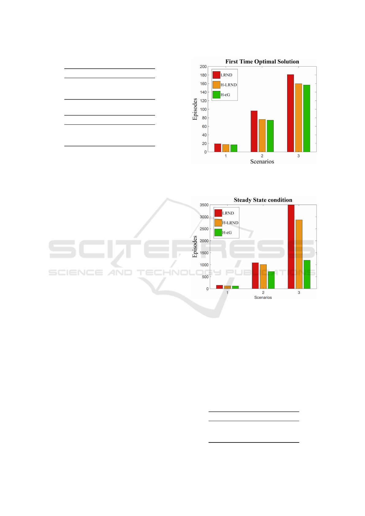
Table 1: Scenario 1.
Algorithm Episodes MP
call
1
st
*
LRND 144 42 20
H-LRND 119 37 18
H-εG 115 34 16
Table 2: Scenario 2.
Algorithm Episodes MP
call
1
st
*
LRND 1079 236 96
H-LRND 1007 218 77
H-εG 717 188 74
4 NUMERICAL VALIDATION
Numerical simulations have been run in order to val-
idate the proposed approach. The robot at hand is a
7-DoF Jaco
2
manufactured by Kinova available in the
robotics lab of the University of Cassino. The im-
plemented motion planning algorithm introduced in
Sect. 3.1 is fully described in (Di Vito et al., 2020). In
detail, the following tasks have been implemented: 1)
Mechanical joint limits avoidance; 2) Self-hit avoid-
ance; 3) Obstacle avoidance with respect to the N
o
ob-
jects and the static ones; 4) Position and orientation of
the arm’s end-effector.
Three different scenarios have been considered
characterised by an increasing number of obstacles:
• Scenario 1. N
o
= 5, ξ
p
= 10. There are ξ
p
= 10
possible sequence from the home to the target
nodes. In particular, since one solution is at level
4 and the other at level > 4, the percentage of opti-
mal solution is 0.3% while the percentage of sub-
optimal solutions is ≈ 3%.
• Scenario 2. N
o
= 10, ξ
p
= 20. One solution is
at level 5 and the other at level > 5, the percent-
age of optimal solution is thus ≈ 10
−5
% while the
percentage of sub-optimal solutions is ≈ 10
−4
%.
• Scenario 3. N
o
= 15, ξ
p
= 20. One solution is at
level 6 and the other at level > 6, the percentage of
optimal solution is ≈ 10
−11
% while the percent-
age of sub-optimal solutions is ≈ 10
−10
%.
For all the learning algorithms (see Sect. 3.2.1), it
is set α = 0.5 and γ = 0.9 and the training is repeated
50 times from scratch. In the case of H-εG algorithm,
it is ε
0
= 1 and ε
min
= 10
−4
in (9). The training ends
whenever condition eq. (11) is satisfied or the maxi-
mum number of episodes E p
max
= 5000 is reached.
As reported in Figure 4, H-εG is the best algorithm
when it comes to reach for the first time the optimal
solution and the interrogation at motion planner sys-
tem. In addition, in Figure 5 is possible to see that
Figure 4: Comparison of three learning policies defined
for each scenario. The average episodes is calculated on
50 training and represent the first time that the target T is
reached through optimal sequence ξ
∗
.
Figure 5: Comparison of convergence between learning
algorithms defined above for each scenario. The average
episodes number is calculated on 50 training.
the algorithm H-εG reach the steady state condition
faster than other algorithms in every scenario for the
ε value chosen. This latter depends on whether that
the ε introduces variation on the learning dynamic.
An additional comparison with the no learning
technique (RND) introduced in Sect. 3.2.1 is here
considered. The implemented algorithm simply ex-
plores the graph resorting to a Breadth First Search
policy by randomly choosing actions until the target
is reached. This is clearly a fast method for a very
Table 3: Scenario 3.
Algorithm Episodes MP
call
1
st
*
LRND 3496 665 181
H-LRND 2868 588 160
H-εG 1189 331 156
ICINCO 2021 - 18th International Conference on Informatics in Control, Automation and Robotics
136

small number of objects, but that becomes quickly in-
tractable. In fact, scenarios 2 and 3 described above
could not be solved in a reasonable amount of time.
Concerning the scenario 1 introduced above, 50 tri-
als were executed and an optimal solution is found in
≈ 60% of cases (100% in the case of learning tech-
niques). In the remaining 40% of trials, all obstacles
are relocated leading to a sub-optimal solutions.
5 CONCLUSION
In this paper, a Reinforcement Learning approach
aimed at performing robotic target relocation in clut-
tered environments is presented. In detail, the pro-
posed method exploits, at a high level, a Q-learning
approach on a dynamic tree structure in order to chose
optimal sequences of obstacles to relocate while, at a
low level, a constraint motion planning is adopted to
plan feasible trajectories for object relocation. Several
exploration strategies of the solution tree, based on
a Breadth-First-Search technique, are presented and
compared, showing that an ε-Greedy approach with
heuristics outperforms other baseline methods and ef-
ficiently solve the problem.
Concerning future work, a pragmatic comprise be-
tween elaboration time and optimality will be sought
by investigating also a Depth-First-Search paradigm,
as well as different and more elaborated reward func-
tions, so as to take into account energetic issues or
other properties of the objects. Similarly, a compari-
son with a Deep Q-Network approach will be done.
REFERENCES
Cheong, S. H., Cho, B. Y., Lee, J., Kim, C., and Nam, C.
(2020). Where to relocate?: Object rearrangement in-
side cluttered and confined environments for robotic
manipulation. arXiv preprint arXiv:2003.10863.
Dantam, N. T., Kingston, Z. K., Chaudhuri, S., and Kavraki,
L. E. (2016). Incremental task and motion planning: A
constraint-based approach. In Robotics: Science and
systems, volume 12. Ann Arbor, MI, USA.
Deng, Y., Guo, X., Wei, Y., Lu, K., Fang, B., Guo, D., Liu,
H., and Sun, F. (2019). Deep reinforcement learning
for robotic pushing and picking in cluttered environ-
ment. In 2019 IEEE/RSJ International Conf. on Intel-
ligent Robots and Systems (IROS), pages 619–626.
Di Lillo, P., Arrichiello, F., Di Vito, D., and Antonelli,
G. (2020). BCI-controlled assistive manipulator: de-
veloped architecture and experimental results. IEEE
Trans. on Cognitive and Developmental Systems.
Di Lillo, P., Simetti, E., Wanderlingh, F., Casalino, G., and
Antonelli, G. (2021). Underwater intervention with
remote supervision via satellite communication: De-
veloped control architecture and experimental results
within the dexrov project. IEEE Trans. on Control
Systems Technology, 29(1):108–123.
Di Vito, D., Bergeron, M., Meger, D., Dudek, G., and An-
tonelli, G. (2020). Dynamic planning of redundant
robots within a set-based task-priority inverse kine-
matics framework. In 2020 IEEE Conf. on Control
Technology and Applications (CCTA), pages 549–554.
Dogar, M. R., Koval, M. C., Tallavajhula, A., and Srini-
vasa, S. S. (2014). Object search by manipulation.
Autonomous Robots, 36(1-2):153–167.
Eppe, M., Nguyen, P. D., and Wermter, S. (2019). From se-
mantics to execution: Integrating action planning with
reinforcement learning for robotic causal problem-
solving. Frontiers in Robotics and AI, 6:123.
G
´
eron, A. (2019). Hands-on machine learning with Scikit-
Learn, Keras, and TensorFlow: Concepts, tools, and
techniques to build intelligent systems. O’Reilly Me-
dia.
Jang, B., Kim, M., Harerimana, G., and Kim, J. W. (2019).
Q-learning algorithms: A comprehensive classifi-
cation and applications. IEEE Access, 7:133653–
133667.
Lagriffoul, F., Dimitrov, D., Bidot, J., Saffiotti, A., and
Karlsson, L. (2014). Efficiently combining task
and motion planning using geometric constraints.
The International Journal of Robotics Research,
33(14):1726–1747.
LeCun, Y., Bengio, Y., and Hinton, G. (2015). Deep learn-
ing. nature, 521(7553):436–444.
Lee, J., Cho, Y., Nam, C., Park, J., and Kim, C. (2019).
Efficient obstacle rearrangement for object manipula-
tion tasks in cluttered environments. In 2019 Inter-
national Conf. on Robotics and Automation (ICRA),
pages 183–189.
Mnih, V., Kavukcuoglu, K., Silver, D., Graves, A.,
Antonoglou, I., Wierstra, D., and Riedmiller, M.
(2013). Playing ATARI with deep reinforcement
learning. arXiv preprint arXiv:1312.5602.
Mohammed, M. Q., Chung, K. L., and Chyi, C. S. (2020).
Review of deep reinforcement learning-based object
grasping: Techniques, open challenges and recom-
mendations. IEEE Access.
Nam, C., Lee, J., Cheong, S. H., Cho, B. Y., and Kim,
C. (2020). Fast and resilient manipulation plan-
ning for target retrieval in clutter. arXiv preprint
arXiv:2003.11420.
Siciliano, B. and Slotine, J.-J. E. (1991). A general frame-
work for managing multiple tasks in highly redundant
robotic systems. In Proc. Fifth International Conf. on
Advanced Robotics (ICAR), pages 1211–1216.
Srivastava, S., Fang, E., Riano, L., Chitnis, R., Russell, S.,
and Abbeel, P. (2014). Combined task and motion
planning through an extensible planner-independent
interface layer. In 2014 IEEE International Conf. on
Robotics and Automation (ICRA), pages 639–646.
Watkins, C. J. and Dayan, P. (1992). Q-learning. Machine
learning, 8(3-4):279–292.
Yuan, W., Hang, K., Kragic, D., Wang, M. Y., and Stork,
J. A. (2019). End-to-end nonprehensile rearrangement
with deep reinforcement learning and simulation-to-
reality transfer. Robotics and Autonomous Systems,
119:119–134.
Task-motion Planning via Tree-based Q-learning Approach for Robotic Object Displacement in Cluttered Spaces
137