An Effective Method for Data Processing of Inertial Measurement Units

Applied to Embedded Systems

Christoph Kolhoff

and Markus Kemper

ZME-Institute, UAS Diepholz (PHWT), Th

uringer Str. 3a, Diepholz, Germany

Keywords:

Bias Error, Gauss-Markov Process, MEMS Error Model.

Abstract:

Autonomous functions for navigation and localization have piqued the attention and interest in many ﬁelds of

science and engineering as automotive, aviation and robotics. Desiring high quantity of autonomous products,

the used components are requested to be cheap. This often lead engineers or developers to apply micro-

electromechanical systems that exhibit large errors. To use these sensors anyway, the acquired data must be

processed online for error reduction. Hence there is a need for an algorithm that is easy to compute. The

aim of this research is to develop a generic algorithm based on a Gauss-Markov process representing the

drifting bias that can be parametrized easily and performs well on real-time systems. Therefore, the error

model imitates the sensor’s output and removing the errors afterwards. Finally, a validation of the suggested

algorithm is performed by comparing processed data of the micro-controller to data processed a posteriori on

a high-performance computer.

1 INTRODUCTION

Autonomous functions are designed to make deci-

sions based on data acquired from sensors without any

human assistance. In foreseeable future autonomous

devices are purposed to take tasks in various sections

of daily life which requires a large large amount of

several accurate sensor data. The commonly used

sensors deliver those precise data but they lead to high

costs of the ﬁnal product. For for low-cost robotic

systems on customer markets the used sensors are re-

quested to be cheap on the one hand and have to pro-

vide data with small errors on the other hand. Hence,

micro-electromechanical systems (MEMS) are the

point of interest in many cases. These kind of sen-

sors exhibit large tolerances and wide ranges of er-

rors as shown in (Kolhoff et al., 2021). In (Titterton

and Weston, 2004) an error model for triaxial IMUs is

given to describe the connectedness between the real

and the measured values. This model contains both,

repeatable (e.g. misalignment, scaling errors, static

bias) and non repeatable (e.g. noise) effects. Looking

at (Titterton and Weston, 2004), it is recommended

to compensate only repeatable errors by applying the

chosen error model. Processing stochastic effects is

not considered by this approach. Acquired data have

to be processed in ”real time” to improve their quality

https://orcid.org/0000-0002-7880-8152

and to reduce errors which leads to the need for sufﬁ-

cient algorithms. Concerning automotive application,

inertial measurement units (IMUs) consisting of ac-

celerometers and gyroscopes are focused to determine

the relevant properties of the vehicle’s actual motion.

To take account of these requirements, the mathemat-

ical structure of the sensor’s behavior has to be known

to be able to develop an algorithm for data processing.

Therefore, an easy model containing misalignment,

constant and drifting bias, noise and nonlinear effects

in triads of sensors is given by (Kuncar et al., 2018).

Additionally, in (Gebre-Egziabher, 2004) some meth-

ods are presented to identify the needed parameters

easily. As a further important requirement, the model

is not just purposed to be parametrized for only one

speciﬁc sensor, but for an entire class of sensors. In

this paper the bias is the focused kind of error because

of its long-time drift characteristics.

In known applications the static component of the

bias is considered only and therefore the entire bias

cannot be compensated completely. Especially when

an integration over time is performed (e.g. by deter-

mining the orientation from the angular velocity), the

resulting errors rise very quickly with time as shown

in (Ramalingam et al., 2009). To design an algorithm

meeting these requirements, the drift of the sensor’s

bias is approximated by a ﬁrst order Gauss-Markov

process (GM) for a single axis, referring to (Gebre-

558

Kolhoff, C. and Kemper, M.

An Effective Method for Data Processing of Inertial Measurement Units Applied to Embedded Systems.

DOI: 10.5220/0010540705580565

In Proceedings of the 18th International Conference on Informatics in Control, Automation and Robotics (ICINCO 2021), pages 558-565

ISBN: 978-989-758-522-7

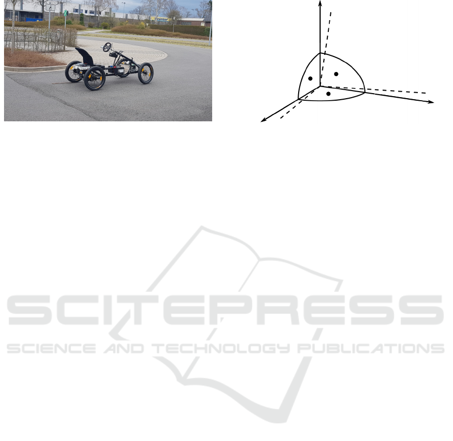
Figure 1: Autonomous ”People-Mover”-Project at UAS

Diepholz.

Egziabher, 2004). In addition to this, the model is

extended by integrating the drifting bias and the al-

gorithm is implemented on a micro-controller after-

wards. Finally, the processed data of the micro-

controller are compared to the same data ﬁltered by

the suggested algorithm on a high-performance com-

puter. It is shown that the mentioned errors are

strongly reduced by the suggested algorithm and the

algorithm is sufﬁcient to operate on real-time sys-

tems. At UAS Diepholz, an fully autonomous low-

cost ”People-Mover” is developed. Figure (1) shows

a photograph while testing sensor systems. The car is

based on an e.Go-Cart and is equipped with sensors

and actuators for self-driving modes. The maximum

speed is 25 to 45 kilometers per hour. Hence, in this

paper, an effective method for data processing of Iner-

tial Measurement Units for the application in low-cost

autonomous systems is proposed.

2 THEORETICAL BACKGROUND

2.1 Generic Error Model for IMUs

The considered sensors exhibit various kinds of er-

rors. Referring to (Titterton and Weston, 2004) a

generic error model for triads of accelerometers and

gyroscopes is denoted in (1) connecting the vector of

measured values

x and real values x. The model con-

tains errors, e.g. due to misalignment represented by

the matrix M.

x = M · x + x

+ x

(1)

This type of error is caused by faulty assembling of

the sensor on the one hand and a lack of orthogo-

nality of the three sensing axes of the IMU resulting

from imperfections in the production process on the

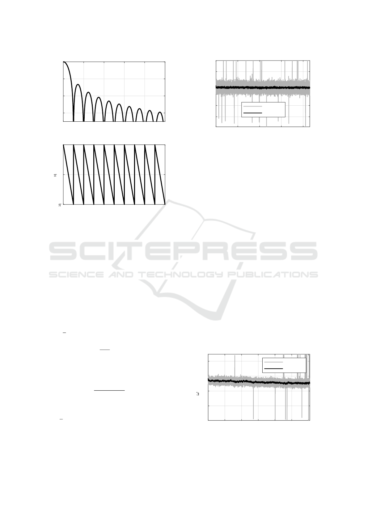
other hand. This is depicted in Figure 2. The acceler-

ations and angular velocities appear along the solid

axes which are aligned orthogonally to each other.

Figure 2: Misalignment of the sensor’s axes.

The sensor measures values along the dashed axes.

Due to the non-orthogonal alignment of the IMU’s

axes the measured values contain amounts of the val-

ues of all solid axes and therefore they appear as linear

combinations of all solid axes’ values. Another rea-

son for this behavior is a fault of sensitivity of each

axis caused by errors in the production process. El-

ements of the major diagonal differing from a value

of one represent errors in sensitivity of the respec-

tive axis. This is caused by the inclination of the

dashed axes to the solid axes. Furthermore, the in-

clination leads to the fact that values measured along

the dashed axes contain amounts of values that are

measured along the other two solid axes. This is rep-

resented by the minor diagonal elements of M which

have commonly small magnitudes (Unsal and Demir-

bas, 2012). The measured values in this case lead to

the assumption that accelerations and angular veloc-

ities occur on axes of the solid coordinate system in

Figure 2 even if there are none in reality. A further

component of the error model is the bias x

. Due to

affection of gravity and imperfections of the internal

structure of the sensor a constant bias x

b,stat

is the ﬁrst

part of x

. Because MEMS have to be powered ex-

ternally, the electric conduction causes heating of the

sensor (W

ustling, 1997). Due to this the internal ge-

ometry of the sensor is diversiﬁed and the bias drifts

over time. This is considered by x

b,drift

, the second

part of x

. As many other sensors MEMS exhibit

noise x

which is assumed as zero-mean white noise

with variance σ

and a band-limit much higher than

the relevant frequencies. The last type of errors is rea-

soned by nonlinear effects x

that occur at high accel-

erations and angular velocities (W

ustling, 1997).

2.2 Characteristics of the Bias

As mentioned in (Ramalingam et al., 2009) and

(Gebre-Egziabher, 2004) the bias b of a sensor con-

tains a constant component b

and a component b

varying with time t as shown in (2) for each axis of

An Effective Method for Data Processing of Inertial Measurement Units Applied to Embedded Systems

559

f [Hz]

-10

-5

G( f )

Figure 3: Power spectral density of a Gauss Markov pro-

cess.

the triaxial sensor.

b(t) = b

+ b

(t) (2)

From the beginning of long-time measured values

the parameter b

is determined easily, whereas the

characterization of b

is often more challenging. As

shown from experimental data in (Kolhoff et al.,

2021), b

can be assumed as exponentially shaped.

Looking at (Gebre-Egziabher, 2004), (Rasmussen and

Williams, 2006) and (Brown and Hwang, 2012), a

very simple method for modeling the drifting bias

with constant ambient temperature is a continuous

ﬁrst order Gauss-Markov process (GM) g deﬁned by

the differential equation shown in (3).

˙g(t) = −T

−1

· g(t) + w

with g(0) = 1 (3)

Herein, T

is the correlation time of the process and

is the Gaussian driving process noise with variance

. The magnitude of the drifting bias is determined

from the end and the beginning of long-time mea-

sured values. Looking at (Brown and Hwang, 2012),

this method is a stationary one ﬁtting well to pro-

cesses that exhibit long correlation times. Due to the

stochastic component the process is not deterministic.

The stochastic component w

is neglected at ﬁrst to

show the general concept of determining T

for a de-

noised process. Therefore, the auto-correlation func-

tion (ACF) Φ is computed from denoised g as shown

in (Gelb et al., 2001). The solution is shown in (4)

with its maximum A

at time lag τ = 0.

Φ(τ) =

∞

−∞

g(t) · g(t + τ) dt = A

· exp(−T

−1

· |τ|)

(4)

All correlation values with a time lag different from

zero are smaller than without time lag due to the

ACF’s exponential shape. This results in decreasing

correlation between samples with increasing time lag

(Brown and Hwang, 2012). Concerning (Gelb et al.,

2001), T

is identiﬁed from a time series of measured

noisy data by the point when the ACF has decayed

to exp(−1) (approximately 36.8 percent) of it’s max-

imum. As to that, when one is able to compensate the

constant and the time-dependent drift of the sensor,

only stochastic effects, scaling errors and cross-axes-

effects will be left.

G( f ) =

2 · A

· T

−1

(2j · π · f )

+ T

−2

(5)

A further need to ensure the usability of the GM

for slowly drifting processes is to look at its power

spectral density function (PSD) G with frequency f .

This can be done best by computing the Fourier-

Transformation of its ACF which leads to the PSD

shown in (5), referring to (Lamon, 2018). The corre-

sponding graph is shown in Figure 3 for T

= 10 mil-

liseconds and A = 1. When looking at the plot it can

be seen that the GM’s energy is concentrated at low

frequencies. Therefore, this model can be used to de-

scribe processes that differ slowly related to its char-

acteristic values as mentioned in (Brown and Hwang,

2012).

2.3 Moving Average Smoothing

For data smoothing the moving average (MA) method

is introduced in (Hyndman, 2010) and (Smith, 1999).

It computes the average ˆz for a time index l from a

connected set of n values from time series z. There

are two versions to use the moving average. One is

to use the two-sided version which means, that the

set contains data before and after the current time in-

dex that the moving average is computed for. At this,

the number of samples before and after the current

time index can be chosen equally or different, result-

ing in a symmetrically or asymmetrically two-sided

moving average. When concerning real-time appli-

cations, only data from previous points of time can

be used for further processing. This version is called

one-sided moving average, its calculation is shown in

(6). Herein it becomes clear, that the oldest value is

-T

1/T

weight

Figure 4: Moving Average ﬁlter.

ICINCO 2021 - 18th International Conference on Informatics in Control, Automation and Robotics

560

0 200 400 600 800 1000

-30

-20

-10

|Z( f )| [dB]

0 200 400 600 800 1000

f [Hz]

- /2

( f ) [rad]

Figure 5: Bode plot for a Moving Average ﬁlter.

dropped and a new one is added to the set before com-

puting the moving average for the new time index.

ˆz(l) =

n−1

∑

k=0

· z

l−k

, l ∈ [k + 1, n − 1], a

= n

−1

(6)

The ﬁlter function in continuous time domain is

shown in Figure 4. Due to the computation from past

values, the use of the moving average causes a phase

delay as shown in (Roscoe and Blair, 2016). In com-

mon applications all considered values are weighted

equally so the ideal moving average ﬁlter is a Finite

Impulse Response (FIR) ﬁlter with duration T and

height

. Transforming (6) into Laplace domain leads

to (7).

Z(s) =

T · s



1 − e

−T ·s



(7)

Because the signal’s frequencies f are the point of in-

terest, a substitution s = 2j·π f with the imaginary unit

j is conducted. The result is denoted in (8).

Z( f ) =

sin(π · f · T )

π · f · T

· e

−j·π· f ·T

(8)

It is well-known, that the moving average is a low-

pass ﬁlter with zero-transmission at the frequencies

with n ∈ N. Its magnitude

Z ( f )

and phase

delay ϕ( f ) are shown in Figure 5 for T = 10 millisec-

onds. This ﬁlter can easily be parametrized because

there is only one parameter T to be chose.

0 200 400 600 800

t [s]

-0.25

-0.2

-0.15

-0.1

-0.05

[m/s

]

raw

denoised

Figure 6: Raw data of the accelerometer.

3 PARAMETRIZE THE ERROR

MODEL AND SUGGEST AN

ALGORITHM FOR ERROR

REDUCTION

To determine the parameters for the suggested error

model data from the IMU is acquired with a sam-

pling frequency of 100 hertz. In ﬁrst instance, mul-

tiple sets of data from all degrees of freedom are ac-

quired from the resting sensor where the three axes

of the accelerometer are aligned matching, opposing

and orthogonal to gravity. For each set of measure-

ment the temperature at the beginning of the measur-

ing process has to be identically and the IMU has to

cool down after completing each set. Exemplary re-

sults for the accelerometer are shown in Figure 6 and

in Figure 7 for the gyroscope. The example of the

accelerometer shows measured data with the y-axis

aligned orthogonally to gravity, so the expected ef-

fective value is zero. The set of raw data contains a

nearly constant difference between the expected value

and the effective mean of the measured values. This

is the bias which is very lightly drifting on this degree

of freedom. In addition to this raw data is affected

by noise and outliers which occur stochastic in time

0 200 400 600 800 1000 1200

t [s]

[°/s]

raw

denoised

Figure 7: Raw data of the gyroscope.

An Effective Method for Data Processing of Inertial Measurement Units Applied to Embedded Systems

561

-5 0 5

real

[m/s

]

-10

-5

meas

[m/s

]

x-axis

y-axis

z-axis

Figure 8: Characteristic lines of the accelerometer.

and intensity. The example of the gyroscope shows

the presence of noise and a drifting bias but no out-

liers. The raw data is post-processed using a high-

order FIR low-pass ﬁlter to reduce the inﬂuence of

noise and stochastic outliers, the results are shown in

the respective ﬁgures. From all taken sets of measure-

ment the effective values at the beginning of the mea-

suring process (static value) and at the end (asymp-

totic value) are determined, the difference of them is

the drifting bias. From these effective values the ele-

ments of the misalignment matrices and the static and

drifting bias are determined. The variance of the raw

data is determined for all degrees of freedom from the

end of each measured set to characterize the occurring

noise. Because the real noise in combination with out-

liers does not represent the assumed white noise the

computed variance is only a rough approximation of

the real noise’s characteristic value. After the asymp-

totic value is removed from the ﬁltered data, only the

exponentially shaped part remains, the ACF is com-

puted for all degrees of freedom of each set from (4)

and the correlation time is determined. Therefore, the

characteristic values for x

and x

in (1) have been de-

termined and are shown in Table 1. Because of multi-

ple alignments of the accelerometer’s axes to gravity,

values from -9.81 meters per square second to 9.81

meters per square second are expected. When the de-

-200 -100 0 100 200

real

[°/s]

-200

-100

100

200

meas

[°/s]

x-axis

y-axis

z-axis

Figure 9: Characteristic lines of the gyroscope.

Algorithm 1: Error reduction by applying the generic error

model.

1 while process running do

2 for j = 1 to 6 do

3 Acquire ˆx

i, j

4 g

i, j



1 −

sampl

c, j



· g

i−1, j

5 x

b,drift,i, j

= g

i, j

· x

b, drift, j

6 x

temp, j

= ˆx

i, j

− x

b,drift,i, j

− x

b, stat, j

7 Computing Moving Average x

from (6)

8 Solve M · x

= x

9 i = i + 1

termined values for the static and drifting bias are re-

moved from the effective values, the elements of the

misalignment matrix M

are determined, the charac-

teristic lines for the accelerometer are shown in Fig-

ure 8 and therefore the model has been parametrized

completely for the accelerometer. The process of

parametrization is done analogous. The only differ-

ence consists of the determination of M

. Therefore,

certain angular velocities are applied to all axes of the

gyroscope on a test rig. The characteristic values are

determined form the acquired data as done for the ac-

celerometer, the characteristic lines for the gyroscope

are shown in Figure 9.

4 SUGGESTED METHOD TO

REDUCE THE ERRORS

The novel method for online-processing of raw val-

ues is listed in Algorithm 1 which is explained for a

time index i. For each degree of freedom (index j)

raw data ˆx

i, j

is acquired from the IMU. Here, ˆx

i,1

, ˆx

i,2

Table 1: Determined range of parameters.

Parameter Values Unit

b,stat,kk

(k ∈

{

x, y, z

}

) -0.17 – 0.026 m/s

b,drift,kk

(k ∈

{

x, y, z

}

) -0.002 – 0.018 m/s

a,k

(k ∈

{

x, y, z

}

) 50 – 167 s

major elem. 0.998 – 1.02 -

minor elem. -0.03 – 0.02 -

a,kk

(k ∈

{

x, y, z

}

) 0.017 – 0.028 m/s

b,stat,kk

(k ∈

{

x, y, z

}

) -0.726 – 2.739

◦

b,drift,k

(k ∈

{

x, y, z

}

) -0.115 – 0.347

◦

ω,kk

(k ∈

{

x, y, z

}

) 1030 – 3760 s

major elem. 0.97 – 1.003 -

minor elem. ≤ 0.001 -

ω,kk

(k ∈

{

x, y, z

}

) 0.01 – 0.013

◦

ICINCO 2021 - 18th International Conference on Informatics in Control, Automation and Robotics

562

0 1000 2000 3000

t [s]

-10

-9.95

-9.9

-9.85

-9.8

-9.75

[m/s

]

raw

online-processed

post-processed

Figure 10: Effect of the algorithm on static bias and scaling

errors.

and ˆx

i,3

are the accelerations in x- y- and z-direction

for the given time index, whereas ˆx

i,4

, ˆx

i,5

and ˆx

i,6

are

the respective angular velocities. In the ﬁrst step of

processing the value of the respective Gauss-Markov

process g

i, j

is computed. Therefore, (3) is solved us-

ing forward Euler integration as shown in (Quarteroni

et al., 2000) with respect to the sampling time T

sampl

afterward. The stochastic component of (3) is ne-

glected. In the second step, the current value of the

drifting bias x

b,drift,i, j

is determined from the respec-

tive Gauss-Markov process and the parameter x

b, drift, j

determined before. Finally, the static bias x

b, stat, j

and

the current drifting bias are removed from the raw

value to gain a value with only small offset. At next

the vector of MA x

is computed for each degree of

freedom due to damping of noise and outliers. The er-

rors due to misalignment are left only. To reduce these

errors, the linear equation system has to be solved

to remove scaling errors and inﬂuences gained from

other axes. All mentioned errors are assumed to be

strongly reduced by now.

500 510 520

t [s]

-0.4

-0.3

-0.2

-0.1

[m/s

]

raw

online-processed

post-processed

Figure 11: Effect of the algorithm on noise and outliers.

0 1000 2000 3000

t [s]

[°/s]

raw

online-processed

post-processed

Figure 12: Performance of the algorithm on drifting bias.

5 EXPERIMENTAL VALIDATION

For the evaluation process Algorithm 1 is imple-

mented onto a micro-controller for all degrees of free-

dom. To ensure that the system is sufﬁcient to operate

under real-time conditions, a 480 megahertz Cortex-

M7 processor with 32-bit architecture is chosen. Raw

and processed data are stored to an external device

directly when the overall set of measurement is com-

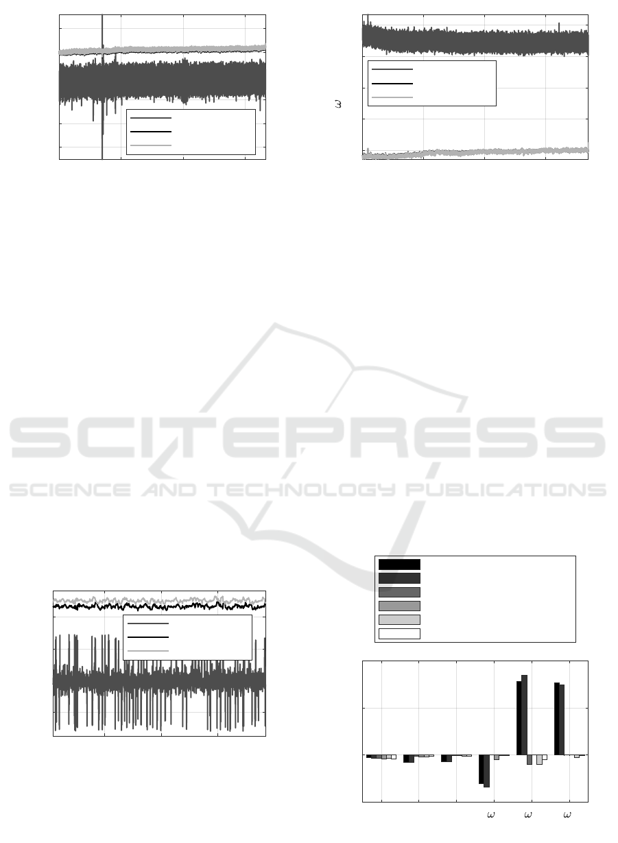
pleted. The results for the accelerometer, which are

shown in Figure 10, are discussed ﬁrst. As it is shown,

the static and asymptotic bias have been strongly re-

duced just as noise and relatively high outliers. In this

example it is shown that the model is valid to reduce

misalignment and static bias errors pretty good. The

remaining error’s magnitude ranges up to 0.03 meters

per square second from the beginning to the end of

the measured set. These errors are denoted in Fig-

ure 13 for all degrees of freedom. The standard de-

z x y z

degree of freedom

-2

error [m/s

or °/s]

initial raw

asymptotic raw

initial processed online

asymptotic processed online

initial processed a posteriori

asymptotic processed a posteriori

Figure 13: Remaining error after processing.

An Effective Method for Data Processing of Inertial Measurement Units Applied to Embedded Systems

563

z x y z

degree of freedom (dof)

0.02

0.04

0.06

0.08

0.1

standard deviation [m/s

or °/s]

raw

post-processed

online-processed

Figure 14: Reduction of the signal’s standard deviation.

viation of the signal is reduced by a factor of 5.7 as

shown in Figure 14 for the respective degree of free-

dom. This exemplary set of measurement shows that

the model is valid to handle misalignment, static bias,

noise and few outliers. Looking at Figure 11 the ef-

fect of the algorithm to strong outliers is presented.

The standard deviation is reduced by a factor of 6

where the absolute intensity of the outliers is smaller

than in Figure 10. In this example it is shown that the

algorithm can also compensate more frequently oc-

curring outliers. The difference between the online-

processed values and the post-processed ones, which

are computed on a high-performance computer after-

ward, is about the same size as in Figure 10. By ap-

plying the suggested algorithm, the remaining mean

error has been reduced down to maximum 6.9 percent

of the error in the gyroscope’s raw data. For the com-

putation of the moving average the last 40 values are

considered for all degrees of freedom. Figure 12

shows the results of the gyroscope: The drifting bias

can be compensated effectively as good. Both, the

online-processed and the post-processed values are

corresponding well with the expected values as it can

be seen in the respective ﬁgures for the results. Here,

the mean value’s highest difference to the expected

value occurs at the beginning of the measurement and

-20 -10 0 10 20

t [ms]

U [V]

acquisition

processing

Figure 15: Elapsed time for acquisition and processing.

decreases with time. Nevertheless the bias of pro-

cessed data is only little drifting and the values that

are processed online are correlating well with the ones

that result from post-processing. Inhere, the cross-

correlation coefﬁcient of the two sets of values is lo-

cated at minimum 98 percent. This shows that the

suggested algorithm is valid to compensate the men-

tioned errors. In Figure 15 the levels of two pins of

the micro-controller are shown. When a new itera-

tion of acquiring and processing is started both pins

are set high. When the respective process is done

the corresponding pin is set low. Considering a fre-

quency of 100 hertz for acquisition and processing the

plot shows that both processes can be performed in

the given time and even for higher sampling frequen-

cies. It can be seen in Figure 15 that the system needs

about 1.4 milliseconds to acquire all data and one pe-

riod containing acquisition and data processing takes

up to 3.3 milliseconds. When analyzing raw and pro-

cessed data it becomes clear that the suggested algo-

rithm is able to effectively reduce the occurring errors

of MEMS meeting real-time conditions.

6 CONCLUSION AND FURTHER

RESEARCH

In this work was shown that the suggested method

is valid to improve the quality of raw data deliv-

ered from MEMS sensors. As a next step for usage

in practical applications similar IMUs can be com-

bined with other sensors like rotary encoders of en-

gines representing odometric data of mobile robots

and cars. Therefore further methods like Kalman Fil-

ters or analogous methods can be used to gain even

higher accuracy of the respective system’s state. In

addition to this the dependencies of all determined

parameters due to the ambient temperature have not

been considered by this work while the temperature

was held constant. During the experimental period the

determined parameters disclosed strong dependencies

of the ambient temperature. Therefore, the suggested

method can be extended by including thermal effects

depending on the ambient temperature. For further

improvement of the method and application in mass

production this method can be automated for integra-

tion in the production process. Therefore, highly au-

tomated test rigs are needed after the fabrication pro-

cess. This test rigs have to take account for aligning

the sensor in every direction with respect to the di-

rection of gravity to acquire data that will be used to

determine the elements of the misalignment matrix of

the accelerometer’s triad. To determine the elements

of the gyroscope’s misalignment matrix the test rigs

ICINCO 2021 - 18th International Conference on Informatics in Control, Automation and Robotics

564

need to rotate the sensor while acquiring data. Other

parameters like noise, static and drifting bias and cor-

relation times can be determined in resting state. Af-

ter all data is acquired an automated computing rou-

tine can be performed in stationary computers and the

determined parameters are stored in non-volatile (e.g.

EEPROM) memory next to the sensor. This leads to a

solution on chip which can be directly integrated into

robots, cars etc.

REFERENCES

Brown, R. G. and Hwang, P. Y. C. (2012). Introduction to

Random Signals and Applied Kalman Filtering with

Matlab Exercises. CourseSmart Series. Wiley.

Gebre-Egziabher, D. (2004). Design and Performance

Analysis of a low-cost aided dead reckoning Naviga-

tor. PhD thesis, Stanford University.

Gelb, A., Kasper, J., Nash, R., Price, C., and Sutherland, A.

(2001). Applied Optimal Estimation. the M.I.T. Press,

Cambridge.

Hyndman, R. (2010). Moving averages. International En-

cyclopedia of Statistical Science, pages 866–869.

Kolhoff, C., Kemper, M., and Olze, M. (2021). Evalua-

tion of low-cost inertial measurement units for appli-

cation in high-volume autonomous vehicles. In Ac-

tuator 2021 - 17th International Conference on New

Actuator Systems and Applications (Actuator 2021),

pages 417–420, Mannheim, Germany.

Kuncar, A., Sysel, M., and Urbanek, T. (2018). Inertial

measurement unit error reduction by calibration us-

ing differential evolution. In 29th DAAAM Interna-

tional Symposium on Intelligent Manufacturing and

Automation, pages 681–686.

Lamon, P. (2018). 3D-Position Tracking and Control for

All-Terrain Robots. Springer, Heidelberg.

Quarteroni, A., Sacco, R., and Saleri, F. (2000). Numerical

Mathematics. Springer, New York.

Ramalingam, R., Ganesan, A., and Shanmugam, J. (2009).

Microelectromechnical systems inertial measurement

unit error modelling and error analysis for low-cost

strapdown inertial navigation system. Defence Sci-

ence Journal, 59(650-658).

Rasmussen, C. and Williams, C. (2006). Gaussian Pro-

cesses for Machine Learning. the M.I.T. Press, Mas-

sachusetts Institute of Technology.

Roscoe, A. and Blair, S. (2016). Choice and properties of

adaptive and tunable digital boxcar (moving average)

ﬁlters for power systems and other signal processing

applications. In 2016 IEEE International Workshop

on Applied Measurements for Power Systems (AMPS),

pages 1–6.

Smith, S. (1999). The Scientist and Engineer’s Guide to

Digital Signal Processing. California Technical Pub-

lishing, San Diego.

Titterton, D. and Weston, J. (2004). Strapdown Inertial

Navigation Technology. The Institution of Electrical

Engineers, 2nd edition.

Unsal, D. and Demirbas, K. (2012). Estimation of deter-

ministic and stochastic imu error parameters. In Pro-

ceedings of the 2012 IEEE/ION Position, Location

and Navigation Symposium, pages 862–868, Myrtle

Beach, SC, USA.

ustling, S. (1997). Hochintegriertes triaxiales Beschle-

unigungssensorsystem. phdthesis, Universit

at Karl-

sruhe. 41.06.01; LK 01; Karlsruhe 1997. (Wis-

senschaftliche Berichte. FZKA. 6003.) Fak. f. Elek-

trotechnik, Diss. v. 7.7.1997.

An Effective Method for Data Processing of Inertial Measurement Units Applied to Embedded Systems

565