Estimating the Frequency of the Sinusoidal Signal using the

Parameterization based on the Delay Operators

Tung Nguyen Khac

, Sergey Vlasov

and Radda Iureva

Faculty of Control Systems and Robotics, ITMO University, Kronversky Pr. 49, St. Petersburg, 197101, Russia

Keywords:

Estimation Parameters, Identiﬁcation Algorithms, Frequency, Sinusoidal Signal, Regressor.

Abstract:

The article presents an algorithm for estimating the frequency of an offset sinusoidal signal. Delay operators

are applied to the measured signal, and a linear regression model is constructed containing the measured

signals and the constant vector depending on unknown frequency. For the vector regression model, the method

cascade reduction is used. A reduction procedure is proposed that allows the original model to be reduced to a

reduced one containing a smaller number of unknown parameters. Finally, using the classical gradient method

was used to compare the efﬁciency of the proposed method.

1 INTRODUCTION

One of the main tasks in the design of automatic con-

trol systems is action alignment of parametrically in-

deﬁnite disturbing inﬂuences on the control object.

In the theory of linear systems, there is an internal

model principle for solving such problems. It is nec-

essary to build models of the reference and disturb-

ing inﬂuences. In the case of harmonic disturbances,

the model parameters will contain unknown frequen-

cies. The initial conditions will be set by unknown

displacement, amplitudes, and phases of the disturb-

ing signal harmonics. In this case, it is necessary to

apply adaptive internal models, which provide para-

metric identiﬁcation possibility of the disturbing sig-

nal.

The task of estimating the parameters of sinu-

soidal signals is fundamental and, in addition to

theoretical signiﬁcance, has wide practical applica-

tion (Stoica et al., 2000). Such problem can arise

during the synthesis of a compensation system for

a parametrically uncertain disturbance (Pyrkin et al.,

2015), for example, in precision displacement sys-

tems (Aphale et al., 2008).

One of the fundamental problems of control the-

ory is the problem of real-time frequency estimation

for a signal consisting of several sinusoids. The prob-

lem is studied in many branches of science: signal

https://orcid.org/0000-0001-6430-1927

https://orcid.org/0000-0002-8345-7553

https://orcid.org/0000-0002-8006-0980

processing, instrument making, adaptive control. The

problem of frequency estimation is widely presented

in practical applications, for example, in precision po-

sitioning systems in nanotechnology (Aphale et al.,

2008), in dynamic positioning systems for vessels ex-

posed to external disturbances such as waves, winds,

and currents (Yohei Takahashi et al., 2007), in power

systems for fault detection (Xia et al., 2012), (Phan

et al., 2016), etc.

As a rule, identifying unknown parameters is

posed from a set of measurements, estimating pa-

rameters in real-time using adaptive control, or com-

pensating for disturbances. The problem of identi-

fying harmonic signal constant frequency has been

well studied over the last decade, and a large number

of real-time algorithms have been developed. Many

approaches solve these problems. The most famous

is the least-squares method and its various modiﬁca-

tions (Lijung.N, 1991). For real-time estimation, it-

erative forms of the least-squares method or gradient

integral algorithms can be used. In (Pyrkin A.A. and

S.A, 2015), an algorithm for continuous-time para-

metric estimation of all parameters of an indeﬁnite

disturbance with a deterministic polyharmonic struc-

ture is presented. Standard gradient estimate is used

for identiﬁcation. In (Vedyakova et al., 2020) algo-

rithm for estimating an asymmetric exponentially de-

caying sinusoid is considered. This problem is a spe-

cial case of the issue considered in this work in the

case of one harmonic in the spectrum of the signal un-

der study. The algorithm is based on the dynamic ex-

pansion of the regressor. In (Aranovskiy et al., 2016),

656

Khac, T., Vlasov, S. and Iureva, R.

Estimating the Frequency of the Sinusoidal Signal using the Parameterization based on the Delay Operators.

DOI: 10.5220/0010536506560660

In Proceedings of the 18th International Conference on Informatics in Control, Automation and Robotics (ICINCO 2021), pages 656-660

ISBN: 978-989-758-522-7

algorithm of frequencies estimation of unbiased poly-

harmonic signal is presented. The algorithm is based

on the use of dynamic expansion of the regressor and

standard gradient estimation and provides exponential

convergence to zero of the estimation error. In (Ara-

novskii, 2008), algorithm of unknown frequency esti-

mation in continuous time of a displaced sinusoidal

signal is considered. The algorithm has noise im-

munity to amplitude-limited measurement noises and

provides asymptotic convergence to zero of the esti-

mation error.

In this article the synthesis of devices for signal

frequency estimation is considered. Parametrization

is proposed to obtain a linear regression model, the

vector of unknown parameters associated with the

original signal parameters. The cascade reduction

method is used to estimate the parameters (Bobtsov

et al., 2010), (Iureva et al., 2020). Conditions are for-

mulated under which the exponential convergence to

zero of the estimation errors is ensured.

This paper is organized as follows: problem state-

ment is described in Section 2; linear regression

model is constructed in Section 3; in Section 4 the es-

timation algorithm is proposed, and exponential con-

vergence of the estimation error to zero is proved; in

Section 5 proposed algorithm computer simulation re-

sults are included conﬁrming the efﬁciency of the ap-

proach and ﬁnally the conclusion.

2 PROBLEM FORMULATION

Consider the measured offset sinusoidal signal:

y(t) = σ + νsin(ωt + ϕ), (1)

where ω ∈ R

is signal frequency, ν ∈ R

– stationary

amplitude, σ ∈ R – is the bias, ϕ ∈ – is rare phase

and the number of signal harmonics y(t). Parameters:

ω, σ, ν, ϕ are considered unknown.

It is required to form estimations

ω(t) of the fre-

quencies that ensure the convergence of the estima-

tion error of

ω(t) = ω −

ω(t) to zero under the fol-

lowing assumptions:

Assumption 1: Signal consists of one harmonic offset.

Assumption 2: Minimum frequency ω and maximum

frequency

ω are known.

3 PARAMETRIZATION

Consider the measurable harmonic signal (1) with ex-

ponentially damped amplitude and bias. On the ﬁrst

step the goal is to ﬁnd linear regression model with

measurable variables and constant parameter associ-

ated with an unknown frequency ω.

Consider two signals:

(t) = y(t − λ),t ≥ λ, (2)

(t) = y(t − 2λ),t ≥ 2λ. (3)

where λ ∈ R

is chosen delay value.

Remark 1: The delay value λ from (2) and (3) should

be chosen such that λ <

The output signals (2) and (3) can be rewritten ex-

plicitly:

(t) = σ + a

νsin(ωt + ϕ) − b

νcos(ωt + ϕ), (4)

(t) = σ + a

νsin(ωt + ϕ) − b

νcos(ωt + ϕ), (5)

where a

= cosωλ, b

= sinωλ, a

= cos2ωλ, b

sin2ωλ and remark that a

= 2a

− 1, b

= 2a

Subtract from (1) multiplied by a

equation (4)

and subtract from (1) multiplied by 2a

− 1 equation

(5). Then is obtain:

y(t) − y

(t) = (a

− 1)σ + b

νcos(ωt + ϕ) (6)

y(t)(2a

− 1) − y

(t) =

= (2a

− 2)σ + 2a

νcos(ωt + ϕ),

(7)

Then subtract from (6) multiplied by 2a

(7) and ob-

tain:

y(t) − y

(t)) − (2a

− 1)y(t) + y

(t) =

= σ(−2a

+ 2), (8)

(t) + y(t) = −2(a

− 1)σ + 2a

(t). (9)

Equation (9) can be written in the form of a linear

regressor with respect to two parameters a

, σ:

ψ(t) = ξ

(t)Θ, (10)

where

ψ(t) = y(t) + y

(t), (11)



(t) 1



, (12)

Θ =



−2(a

− 1)σ







. (13)

4 PARAMETER ESTIMATION

In the previous section linear regression model (10)

was gained. In this section the method for param-

eter estimation is proposed. Estimation algorithm

is presented based on the cascade reduction method

(Bobtsov et al., 2010).

Estimating the Frequency of the Sinusoidal Signal using the Parameterization based on the Delay Operators

657

Figure 1: Block diagram of the algorithm (18).

In this case we sequentially integrate equation (9),

i.e.:

(τ) + y (τ)) dτ =

= θ

(τ)dτ + θ

dτ, (14)

Introduce the notation:

(t) =

(τ) + y(τ))dτ,

(t) =

dτ,

(t) =

(τ)dτ.

and sequentially ﬁrst divide by α

(t), and then differ-

entiate the last relation. Then get:

−1

− α

−2

= θ

(

−1

− α

−2

). (15)

Divide (15) into two parts by α

−2

, and obtain:

− α

= θ

(

− α

). (16)

Introduce the following notation: β

−

, β

− α

Then equation (16) takes the next form:

(t) = θ

(t). (17)

whence follows an identiﬁcation algorithm in the

form:

(t) = −γ

(t)β

(t) + γ

(t)β

(t). (18)

where γ

∈ R

is the chosen constant that provides ex-

ponential convergence of the estimation error to zero.

From (17) and (18) can be obtained the differential

equations for errors checking:

(t) = θ

−

(t).

Frequency Estimation

It follows from (18) that:

ω(t) =

arccos

. (19)

Figure 2: Block diagram of the algorithm (22).

Since the function domain (19) is the subset of R,

it is necessary to put some restrictions on it

(t). Un-

der Assumption possible values of θ

satisfying the

inequality:

2cos

ωλ ≤ θ

≤ 2cosωλ. (20)

Rewrite estimation for

, which would satisfy the

next equation:

(t) = Pr(−γ

(t)β

(t) + γ

(t)β

(t)). (21)

The projection Pr(∗) allows condition (20) to be sat-

isﬁed so that the estimation remains qualitatively the

same (P.A.Loannou, 2012).

5 NUMERICAL EXAMPLES

In this section the simulation results are presented.

These results illustrate the efﬁciency of proposed es-

timation algorithm. All simulations have been per-

formed in MATLAB Simulink.

Let us compare the proposed algorithm with other

identiﬁcation. The gradient descent method was taken

as an example.

The device for estimating parameters based on

gradient descent has the form:

Θ = Kξ



ψ − ξ



, (22)

where K ∈ R

is the chosen constant that provides

exponential convergence of the estimation error to

zero. Different signal was taken to check the algo-

rithm operation. This signal belongs to earlier con-

sidered algorithm for two different harmonics: y(t) =

4 + 2sin(2t + 2) and y(t) = 5 + 2sin(4t + 1). Delay

statements are used with the following delay values:

Method Cascade Reduction: γ

= 1, γ

= 20 and λ =

0.1, 0.3, 0.5.

The simulation results are shown in ﬁgures 3, 4, 5,

Method Gradient Descent: K = 0.1, K = 0.5 and λ =

0.1, 0.3, 0.5.

The simulation results are shown in ﬁgures 7, 8, 9,

10.

ICINCO 2021 - 18th International Conference on Informatics in Control, Automation and Robotics

658

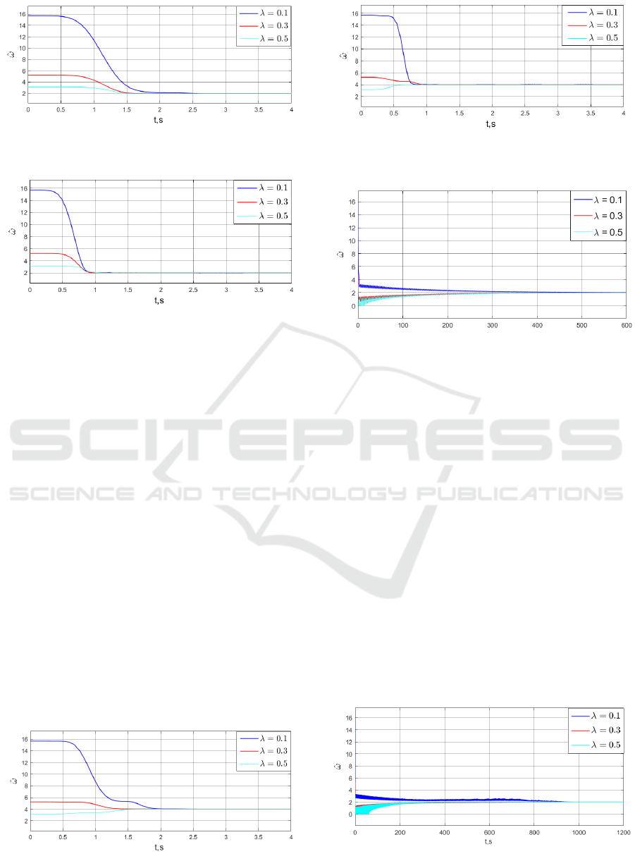
Figure 3: Parameter estimation transients for signal y(t) =

4 + 2sin(2t + 2) at γ

= 1 (Method Cascade Reduction).

Figure 4: Parameter estimation transients for signal y(t) =

4 + 2sin(2t + 2) at γ

= 20 (Method Cascade Reduction).

Remark 2: There is an optimal value at which the

speed is maximum in the gradient method, and for the

cascade reduction method, show that with an increase

in the value, the convergence time is much faster, the

speed can be increased inﬁnitely. At the same time,

looking at the diagrams, we can see that when chang-

ing the delay operator, the method of reduction is al-

most unchanged, but for the gradient method, the con-

vergence time increases quite a lot and the overshoot

increases.

For the case of unknown parameters, numerical

modeling was carried out, which illustrated that when

using the cascade reduction method, the oscillations

in the parameter estimates were signiﬁcantly lower,

and the response time was much faster than when us-

ing the gradient descent method. For the slope reduc-

tion method in both cases, the temporary time to esti-

mate the signal parameters is 450 seconds, compared

with 2 second for the cascading method.

The simulation results show that when using the

cascade reduction algorithm, the parameter estimates

are signiﬁcantly lower and the response time is much

Figure 5: Parameter estimation transients for signal y(t) =

5 + 2sin(4t + 1) at γ

= 1 (Method Cascade Reduction).

Figure 6: Parameter estimation transients for signal y(t) =

5 + 2sin(4t + 1) at γ

= 20 (Method Cascade Reduction).

Figure 7: Parameter estimation transients for signal y(t) =

4 + 2sin(2t + 2) at K = 0.1 (Method Gradient Descent).

faster than when using the gradient method, and there

is almost no overshoot when using the cascade reduc-

tion method. Thus, the cascade reduction method may

be preferable for use in practical problems.

6 CONCLUSIONS

In the article the problem harmonic signal parame-

ters deﬁnition is considered. New parameterization

method based on operator delay application to mea-

surable signal is applied to construct linear regression

model. Methods for producing estimates of the fre-

quency of a harmonic signal are presented, making it

possible to obtain estimates of the parameters at a pre-

determined time. Computer simulation has been car-

ried out to illustrate the performance, demonstrating

the parametric convergence of the algorithm variable

(19), (22) to the correct value. Obtained algorithms

Figure 8: Parameter estimation transients for signal y(t) =

4 + 2sin(2t + 2) at K = 0.5 (Method Gradient Descent).

Estimating the Frequency of the Sinusoidal Signal using the Parameterization based on the Delay Operators

659

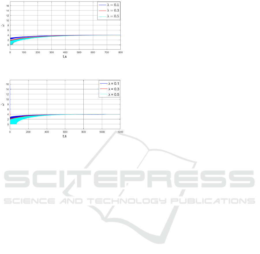
Figure 9: Parameter estimation transients for signal y(t) =

5 + 2sin(4t + 1) at K = 0.1 (Method Gradient Descent).

Figure 10: Parameter estimation transients for signal y(t) =

5 + 2sin(4t + 1) at K = 0.5 (Method Gradient Descent).

are supposed to compensate vertical inertial accelera-

tions in estimating gravity anomalies on moving ob-

ject. Future investigations will be devoted to extend-

ing the methodology to the case of multisinusoidal

signal estimation.

REFERENCES

Aphale, S. S., Bhikkaji, B., and Moheimani, S. (2008).

Minimizing scanning errors in piezoelectric stack-

actuated nanopositioning platforms. Nanotechnology,

IEEE Transactions on, 7:79 – 90.

Aranovskii, S.V., B. A. K. A. (2008). Identiﬁcation of fre-

quency of a shifted sinusoidal signal.

Aranovskiy, S., Bobtsov, A., Romeo, O., and Anton, P.

(2016). Improved transients in multiple frequencies

estimation via dynamic regressor extension and mix-

ing. IFAC-PapersOnLine, 49.

Bobtsov, A., Kolyubin, S., and Pyrkin, A. (2010). Com-

pensation of unknown multi-harmonic disturbances in

nonlinear plant with delayed control. Automation and

Remote Control, 71:2383–2394.

Iureva, R., Kremlev, A., Subbotin, V., Kolesnikova, D.,

and Andreev, Y. (2020). Digital twin technology for

pipeline inspection. pages 329–339.

Lijung.N (1991). Systems identiﬁcation. theory for the user.

19(2):432.

P.A.Loannou, J. S. (2012). Robust adaptive control. page

821.

Phan, A. T., Hermann, G., and Wira, P. (2016). A new state-

space for unbalanced three-phase systems: Applica-

tion to fundamental frequency tracking with kalman

ﬁltering. pages 1–6.

Pyrkin, A., Bobtsov, A., Nikiforov, V., Kolyubin, S.,

Vedyakov, A., Borisov, O., and Gromov, V. (2015).

Compensation of polyharmonic disturbance of state

and output of a linear plant with delay in the control

channel. Automation and Remote Control, 76:2124–

2142.

Pyrkin A.A., Bobtsov A.A., V. A. and S.A, K. (2015). Ro-

bust and adaptive systems.

Stoica, P., Hongbin Li, and Jian Li (2000). Amplitude esti-

mation of sinusoidal signals: survey, new results, and

an application. IEEE Transactions on Signal Process-

ing, 48(2):338–352.

Vedyakova, A., Vedyakov, A., Bobtsov, A., and Pyrkin, A.

(2020). Drem-based parametric estimation of bias-

affected damped sinusoidal signals *. pages 214–219.

Xia, Y., Douglas, S. C., and Mandic, D. P. (2012). Adaptive

frequency estimation in smart grid applications: Ex-

ploiting noncircularity and widely linear adaptive esti-

mators. IEEE Signal Processing Magazine, 29(5):44–

54.

Yohei Takahashi, Shigeki Nakaura, and Mitsuji Sampei

(2007). Position control of surface vessel with un-

known disturbances. pages 1673–1680.

ICINCO 2021 - 18th International Conference on Informatics in Control, Automation and Robotics

660