Multi-target Optimal Control Problems for a Tentacle-like Soft
Manipulator
Simone Cacace
1
, Anna Chiara Lai
2 a
and Paola Loreti
2
1
Dipartimento di Matematica e Fisica, Universit
`
a degli Studi Roma Tre, Largo S. Murialdo, 1, 00154 Roma, Italy
2
Dipartimento di Scienze di Base e Applicate per l’Ingegneria, Sapienza Universit
`
a di Roma, Via A. Scarpa, 16, 00161
Roma, Italy
Keywords:
Soft Manipulators, Control Strategies, Reachability, Multi-target Problems, Optimal Control.
Abstract:
We investigate the optimality of the configurations of a tentacle-like soft manipulator ensuring the contact with
a target object, while avoiding an obstacle. The main novelty consists in treating the contact sub-region of the
manipulator as an unknown of the problem and, at the same time, in allowing the target to be disconnected.
We set the optimization problem in full generality, then we focus on the case of a multi-target problem, in
which the goal is to simultaneously reach a finite set of points. Numerical simulations complete the paper.
1 INTRODUCTION
In this paper, we investigate the optimality of the
configurations of a tentacle-like soft manipulator en-
suring the simultaneous contact with several, discon-
nected targets, and obstacle avoidance. In (Cacace
et al., 2020a), we introduced a control model for a soft
manipulator, modelled as an inextensible string sub-
ject to a bending moment, a curvature constraint and
a pointwise curvature control. The dynamics of the
manipulator was then studied in an optimal control
theoretic perspective, with the purpose of character-
izing optimal control strategies for several tasks, in-
cluding optimal reachability problems (Cacace et al.,
2019a), obstacle avoidance (Cacace et al., 2020b; Ca-
cace et al., 2021) and grasping problems (Cacace
et al., 2019b).
In particular, in (Cacace et al., 2019b) it was ad-
dressed the problem, in a stationary setting, to touch
the boundary of a target object with a prescribed por-
tion of the manipulator, while avoiding interpenetra-
tion and minimizing a quadratic cost on the controls.
Here we move a step forward in this direction, let-
ting the manipulator touch some fixed points on the
boundary of the target object using contact points
which optimize a given integral cost. Hence the main
novelty consists in treating the contact sub-region of
the manipulator as an unknown of the problem and,
at the same time, in allowing the target to be discon-
a
https://orcid.org/0000-0003-2096-6753
nected. For instance, if the target is a set of points
(possibly on the boundary of the obstacle), we are
looking for an optimal, obstacle avoiding configura-
tion of the manipulator which ”interpolates” the set of
the target points. We numerically solve several opti-
mal problems in this scenario, whereas the theoretical
framework is set in full generality.
The paper is organized as follows. In Section
2, we recall our model for tentacle-like soft manip-
ulators and the associated equilibria. In Section 3,
we present the multi-target optimal control problem,
the corresponding optimality system, and an iterative
method for its solution. In Section 4, we discuss
the numerical approximation and implementation of
the proposed algorithm, then we show the results of
the numerical experiments. Finally, in Section 5, we
present our conclusions.
We refer to (Michalak et al., 2014; Rus and Tolley,
2015; Laschi and Cianchetti, 2014; George Thuruthel
et al., 2018) and the reference therein for a general
introduction on soft robotics and related motion plan-
ning problems. The paper (Hughes et al., 2016) sur-
veys grasping problems for soft-manipulators, where
we refer to the papers (Bobrow et al., 1983; Wang
et al., 2016) for an optimal control theoretic approach
to constrained reachability problems. The model dis-
cussed here was earlier introduced in (Cacace et al.,
2020a), related references include (Jones and Walker,
2006; Kang et al., 2011; Lai and Loreti, 2014; Lai
et al., 2016; Laschi et al., 2012).
Cacace, S., Lai, A. and Loreti, P.
Multi-target Optimal Control Problems for a Tentacle-like Soft Manipulator.
DOI: 10.5220/0010533400390048
In Proceedings of the 18th International Conference on Informatics in Control, Automation and Robotics (ICINCO 2021), pages 39-48
ISBN: 978-989-758-522-7
Copyright
c
 2021 by SCITEPRESS – Science and Technology Publications, Lda. All rights reserved
39

2 MODELING A
TENTACLE-LIKE
SOFT-MANIPULATOR
In (Cacace et al., 2020a), we introduced a control
model for a soft manipulator inspired by the morphol-
ogy of an octopus tentacle. We considered a three-
dimensional body with an axial symmetry, a non-
uniform thickness and a fixed endpoint. We assumed
the device to be subject to an inextesibility constraint
(preventing longitudinal stretching) and to a bend-
ing moment, constraint and control. The bending of
the device is hence opposed by a natural resistance,
represented by the bending moment; the bending is
however bounded by a non-uniform threshold repre-
sented by the bending constraint and, finally, the con-
troller can force the bending pointwise. Exploting
axial symmetry, we restricted the investigation to the
symmetry axis, by ending up in a planar dynamics and
an unidimensional problem. From a physical point
of view, such an axis is modelled as an inextensible
string, whose mass represents the mass of the whole
manipulator. Also bending constraints (and controls)
of the manipulator are projected on the axis: they are
identified by suitably weighted curvature constraints,
see (Cacace et al., 2019a) for details on this projec-
tion. In particular, the bending constraint is trans-
lated into forcing the curvature of the axis under a
fixed (non-uniform) threshold ω; the bending control
is translated into forcing the signed curvature to the
quantity ωu, where u ∈ [−1,1] is the control map.
Curvature constraints and control, as well as the bend-
ing moment, are embedded via penalization, whereas
the inextensibility constraint is exact.
The unknowns of our problem are the curve
q(s,t) : [0,1] ×R
+
→ R
2
parametrizing the symmetry
axis of the manipulator in arclength coordinates, and
the associated inextensibility multiplier σ(s,t) ∈ R.
We denote by q
s
, q
ss
, q
tt
partial derivatives in space
and time respectively. The quantity |q
ss
| represents
the curvature of q, whereas the product q
s
× q
ss
:=
q
s
·q
⊥
ss
represents the signed curvature, where the sym-
bol q
⊥
ss
denotes the counter-clockwise orthogonal vec-
tor to q
ss
. With these notations, we summarize the
constraints described above in Table 1, that we recall
from (Cacace et al., 2019a). We refer to Figure 1-(b) –
Figure 6-(b) for an example of the curvature threshold
ω and some (optimal) control functions u.
Then, the evolution of q (and of the corresponding
inextensibility multiplier σ : [0,1] × [0,+∞) → R) is
obtained, via the least action principle, by the follow-
ing Lagrangian:
Table 1: Exact constraint equations and related elastic po-
tentials derived from penalty method. The functions ν and
µ represent non-uniform elastic constants.
Constraint Constraint Penalization
equation elastic potential
Inextensibility |q
s
| = 1 None
Curvature |q
ss
| ≤ ω ν(|q
ss
|
2
− ω
2
)
2
+
Control q
s
× q
ss
= ωu µ (ωu − q
s
× q
ss
)
2
L(q,σ) : =
Z
1
0

1
2
ρ|q
t
|
2
| {z }
kinetic energy
−
1
2
σ(|q
s
|
2
− 1)
| {z }
inextensibility constr.
−
1
4
ν

|q
ss
|
2
− ω
2

2
+
| {z }
curvature constr.
−
1
2
ε|q
ss
|
2
| {z }
bending moment
−
1
2
µ(ωu − q
s
× q
ss
)
2
| {z }
curvature control

ds ,
Equations of motions are explicitly derived in (Ca-
cace et al., 2020a), to which we also refer for a more
rigorous justification of the definition of L. Here we
are most interested in recalling the stationary config-
urations associated to above Lagrangian. Assuming
the technical condition µ(1) = µ
s
(1) = 0, the shape of
the manipulator at the equilibrium is the solution q of
the following second order controlled ODE:







q
ss
=
¯
ωuq
⊥
s
in (0,1)
|q
s
|
2
= 1 in (0,1)
q(0) = (0,0)
q
s
(0) = (0,−1).
(1)
where
¯
ω := µω/(µ + ε) is the effective threshold due
to the competition between the bending moment and
the curvature control.
3 THE MULTI-TARGET
OPTIMAL CONTROL
PROBLEM
Let Ω
0
be an open subset of R
2
representing the ob-
stacle, and let Ω
1
⊂ R
2
\ Ω
0
be a closed target set –
we also allow the case Ω
1
⊂ ∂Ω
0
. We consider the
following optimal control problem
minG, subject to (1) and to |u| ≤ 1, (2)
where
G(q,u) : =
1
2
Z
1
0
u
2
ds
+
1
2τ
0
Z
1
0
W
0
(q(s))ds +
1
2τ
1
Z
1
0
W
1
(q(s))µ
0
(s)ds
,
(3)
ICINCO 2021 - 18th International Conference on Informatics in Control, Automation and Robotics
40

is the cost functional for the multi-target problem,
for some positive penalty parameters τ
0
and τ
1
. The
first integral term of G is a quadratic cost on the con-
trols, which is related via (1) to the curvature of the
manipulator. The potential W
0
: R
2
→ R is a positive
function supported in Ω
0
, and acting as an obstacle,
i.e. forcing all the points of the manipulator to move
outside Ω
0
. Similarly, W
1
: R
2
→ R is a positive po-
tential supported in the complement Ω
c
1
, so that the
third term in (3) penalizes the distance from the target
Ω
1
, attracting points according to µ
0
, a non negative
weight describing which parts of the manipulator are
preferred for touching the target.
In (Cacace et al., 2019b; Cacace et al., 2021),
problem (2) was investigated and then numerically
solved when Ω
1
= ∂Ω
0
and µ
0
is prescribed. Here,
we move further, by considering Ω
1
:= {p
1
,... , p
N
},
namely a set of N fixed points, possibly located on
∂Ω
0
. Moreover, we introduce N additional unknowns
S = {s
1
,... , s
N
} ∈ I
γ
:= [γ,1 − γ], i.e. real numbers
belonging, for some small parameter γ > 0, to the in-
terior of the parametrization interval of the manipula-
tor, and we assume that µ
0
(s) =
∑
N
i=1
δ
s
i
(s) is a Dirac
measure concentrated on S. With these choices, the
functional G in (3) takes the form
G(q,S) : =
1
2
Z
1
0
1
¯
ω
2
(s)
|q
ss
|
2
ds
+
1
2τ
0
Z
1
0
W
0
(q(s))ds +
1
2τ
1
N
∑
i=1
|q(s
i
) − p
i
|
2
,
(4)
where we used (1) to replace the control term by the
curvature of the manipulator, weighted by
¯
ω. Then,
the optimal control problem (2) now consists in min-
imizing G with respect to q and S, subject to the con-
straints q(0) = (0, 0), q
s
(0) = (0,−1), |q
s
(s)|
2
= 1,
|q
ss
| ≤
¯
ω for s ∈ (0,1) and s
i
∈ I
γ
for i = 1,. . . , N.
To obtain necessary optimality conditions, we first
relax the inequality constraint on the curvature |q
ss
| ≤
¯
ω, by introducing a so called slack variable, namely
we impose the equivalent (and simpler to treat) equal-
ity constraint |q
ss
|
2
−
¯
ω
2
+z = 0 with z ≥ 0. Then, we
introduce the following augmented Lagrangian
L(q,σ,S,z, λ) :=G (q,S) +
1
2
Z
1
0
σ(|q
s
|
2
− 1)ds
+
1
2
Z
1
0
λ(|q
ss
|
2
−
¯
ω
2
+ z)ds
+
1
4ρ
λ
Z
1
0
(|q
ss
|
2
−
¯
ω
2
+ z)
2
ds ,
(5)
where σ is again an exact Lagrange multiplier for
the inextensibility constraint, while λ and ρ
λ
> 0
are respectively the multiplier and penalty parame-
ter related to the relaxed constraint on the curva-
ture. In this setting, our optimal control problem
is equivalent to the optimization of L, which can
be performed employing the method of multipliers
((Hestenes, 1969; Powell, 1969), see also (Chris-
tian Kanzow and Wachsmuth, 2018) and the refer-
ences therein for the infinite-dimensional case), iter-
ating on k ≥ 0 up to convergence

















( ˜q
(k+1)
,
˜
σ
(k+1)
,
˜
S
(k+1)
, ˜z
(k+1)
) =
arg min
q, σ
S ∈ I
γ
, z ≥ 0
L(q,σ,S,z, λ
(k)
)
λ
(k+1)
= λ
(k)
+
1
ρ
λ
(| ˜q
(k+1)
ss
|
2
−
¯
ω
2
+ ˜z
(k+1)
).
(6)
Here, the dependence on z can be dropped. Indeed,
the optimization with respect to z ≥ 0 yields the fol-
lowing variational inequality
Z
1
0
(λ
(k)
ρ
λ
+ |q
ss
|
2
−
¯
ω
2
+ z)(v − z)ds ≥ 0 , ∀v ≥ 0,
and its solution is given pointwise by
z = z(q,λ
(k)
) = max
n
−λ
(k)
ρ
λ
− |q
ss
|
2
+
¯
ω
2
,0
o
.
This allows to reduce the update formula for the mul-
tiplier in (6) to
λ
(k+1)
= max

λ
(k)
+
1
ρ
λ
(| ˜q
(k+1)
ss
|
2
−
¯
ω
2
),0

. (7)
On the other hand, the solution ( ˜q
(k+1)
,
˜
σ
(k+1)
,
˜
S
(k+1)
)
of the optimization sub-problem for the reduced La-
grangian
L
(k)
(q,σ, S) := L(q,σ, S,z(q, λ
(k)
),λ
(k)
) (8)
satisfies the following optimality system










































Λ
(k)
(q
ss
)q
ss

ss
− (σq
s
)
s
+
1
τ
0
∇W
0
(q(s))
+
1
τ
1
∑
N
i=1
(q(s) − p
i
)δ
s
i
(s) = 0 in (0,1)
|q
s
|
2
= 1 in (0,1)
1
τ
1
(q(s
i
) − p
i
) · q
s
(s
i
)(w
i
− s
i
) ≥ 0 , ∀w
i
∈ I
γ
i = 1,..., N
q(0) = 0, q
s
(0) = (0, −1)
q
ss
(1) = 0, q
sss
(1) = 0 ,
σ(1) = 0 ,
(9)
with
Λ
(k)
(q
ss
) :=
1
¯
ω
2
+ max

λ
(k)
+
1
ρ
λ
(|q
ss
|
2
−
¯
ω
2
),0

.
The first equation and the boundary conditions in
(9) emerge from the optimization of L
(k)
with respect
Multi-target Optimal Control Problems for a Tentacle-like Soft Manipulator
41

to q. We refer to (Cacace et al., 2020a) for details, and
we remark that the novelty in this paper is the obstacle
repulsion –which is provided by the gradient of the
potential W
0
– and the contact set S appearing in the
last term of the equation, a force field whose source
points attract single particles of the manipulator.
The second equation is the inextensibility con-
straint, recovered by the optimization of L
(k)
with re-
spect to σ.
Finally, the optimization with respect to s
i
∈ I
γ
for i = 1,. . . , N provides the variational inequalities
in (9). Note that, if for some i the optimal s
i
falls in
the interior of I
γ
, then
1
τ
1
(q(s
i
) − p
i
) · q
s
(s
i
) = 0, i = 1,. . . , N . (10)
From a geometric point of view, this condition is
clearly satisfied, as τ
1
→ 0, if s
i
realizes a perfect con-
tact q(s
i
) = p
i
, but since the contact is imposed via
penalization with τ
1
<< 1, condition (10) weakens in
requesting a null projection of (q(s
i
) − p
i
) on the tan-
gent vector q
s
(s
i
).
We now employ a projected gradient descent
method for the approximation of the solution of (9).
To this end, we collect the partial Fr
´
echet derivatives
of L
(k)
in
L
0(k)
(q,σ,S) =
















Λ
(k)
(q
ss
)q
ss

ss
− (σq
s
)
s
+
1
τ
0
∇W
0
(q(s))
+
1
τ
1
∑
N
i=1
(q(s) − p
i
)δ
s
i
(s)
1
2
(|q
s
|
2
− 1)
1
τ
1
(q(s
1
) − p
1
) · q
s
(s
1
)
.
.
.
1
τ
1
(q(s
N
) − p
N
) · q
s
(s
N
)















,
(11)
where the last N entries correspond to the uncon-
strained cases (10) for the variational inequalities in
(9).
Then, given an initial guess (q
(0)
,σ
(0)
,S
(0)
), we
iterate on n ≥ 0 up to convergence
















q
(n+1)
σ
(n+1)
¯
S
(n+1)



=



q
(n)
σ
(n)
S
(n)



− αL
0(k)
(q
(n)
,σ
(n)
,S
(n)
),
S
(n+1)
= Π
I
γ

¯
S
(n+1)

,
(12)
where α > 0 is the step size and
Π
I
γ
(·) = min{max{·,γ}, 1 − γ}
is the component-wise projection on I
γ
ensuring a
feasible contact set at each iteration.
We conclude this section by remarking that, at
least at a formal level, the presented analysis has been
carried on in an infinite-dimensional setting, but its
rigorous justification and the proof of convergence re-
sults for both the method of multipliers and the pro-
jected gradient descent method is a very delicate task
which is still under development.
4 NUMERICAL
APPROXIMATION AND
SIMULATIONS
We briefly discuss the relevant steps for the approxi-
mation of the multi-target problem, then we build our
algorithm for an actual implementation. Finally, we
present the results for several numerical experiments,
showing the effectiveness of the proposed approach.
After introducing a uniform grid on the
parametrization interval of the manipulator, the
discretization of the derivatives appearing in (11) is
performed using standard finite differences, while the
boundary conditions in (9) can be handled adding
suitable ghost nodes at the end points. Moreover,
we observe that the contact values S = {s
1
,... , s
N
}
need not to be discretization nodes, hence the corre-
sponding contact points q(s
1
),. . . , q(s
N
) in (11) are
reconstructed via linear interpolation of neighboring
grid nodes. We also use a rectangular quadrature rule
to evaluate all the integrals in the Lagrangian L
(k)
(see (8), (5) and (4)). Finally, the penalty parameters
τ
0
, τ
1
and ρ
λ
must be chosen very small in order
to enforce, respectively, the obstacle avoidance,
the contact with the target points and the curvature
constraint. Here we use a continuation method to
slowly decrease these parameters, by means of a
scaling factor χ < 1. For simplicity, we embed
this update in the iteration step for the method of
multipliers (6).
We have to remark that, despite its straightfor-
ward implementation, the gradient descent method is
known to suffer a severe restriction on the step size
α, hence it requires a very large number of iterations
to reach convergence. Computational efforts can be
mitigated introducing more sophisticated techniques,
such as an inexact line-search strategy based on the
Armijo–Goldstein condition to obtain an almost opti-
mal α. Alternatively, we can directly apply a Newton
method to the problem L
0(k)
= 0, but it requires the
computation of the second Fr
´
echet derivative L
00(k)
,
which is very involved in the present setting. This
goes beyond the scope of the paper and we omit the
details.
ICINCO 2021 - 18th International Conference on Informatics in Control, Automation and Robotics
42

We finally build the following algorithm.
Algorithm 1.
1: Assign the obstacle Ω
0
, the potential W
0
, the curvature
threshold
¯
ω, the N target points {p
1
,. .. , p
N
} ∈ ∂Ω
0
,
the interval I
γ
, an initial guess (q
]
,σ
]
,S
]
), initial penalty
parameters τ
0
,τ
1
,ρ
λ
, a step size α, a scaling factor χ <
1 and a tolerance tol > 0.
2: Set k ← 0
3: Set ( ˜q
(k)
,
˜
σ
(k)
,
˜
S
(k)
) ← (q
]
,σ
]
,S
]
)
4: Compute L
new
out
= L
(k)
(q
]
,σ
]
,S
]
)
5: Set L
new
in
← L
new
out
6: repeat (Method of multipliers)
7: Set n ← 0
8: Set (q
(n)
,σ
(n)
,S
(n)
) ← ( ˜q
(k)
,
˜
σ
(k)
,
˜
S
(k)
)
9: Set L
old
out
← L
new
out
10: repeat (Projected gradient descent method)
11: Set L
old
in
← L
new
in
12: Compute (q
(n+1)
,σ
(n+1)
,S
(n+1)
) using (12)
13: Compute L
new
in
= L
(k)
(q
(n+1)
,σ
(n+1)
,S
(n+1)
)
14: Set n ← n + 1
15: until


L
new
in
− L
old
in


< tol
16: Set ( ˜q
(k+1)
,
˜
σ
(k+1)
,
˜
S
(k+1)
) ← (q
(n)
,σ
(n)
,S
(n)
)
17: Compute λ
(k+1)
using (7)
18: Set τ
0
← χτ
0
19: Set τ
1
← χτ
1
20: Set ρ
λ
← χρ
λ
21: Set L
new
out
← L
new
in
22: Set k ← k + 1
23: until


L
new
out
− L
old
out


< tol
Table 2: Obstacle and target settings. Q
l
(c) denotes the
square of side l = 0.3 and center c = (0.2,−0.3).
Test # Ω
0
Ω
1
1
/
0 {(0.25,−0.7)}
2
/
0 {(0.094,−0.406),(0.094,−0.406)}
3
/
0 {(0.05,−0.3),(0.2,−0.45), (0.35, −0.3)}
4
/
0 {(0.1,−0.3),(0.2,−0.45), (0.3, −0.3)}
5
/
0 {(0.135,−0.3),(0.2,−0.5), (0.265, −0.3)}
6 Q
l
(c) {(0.05, −0.15),(0.05,−0.45),(0.35,−0.45)}
7 Q
l
(c) {(0.05, −0.3),(0.2,−0.45),(0.35,−0.3)}
Let us now define the settings for our numeri-
cal experiments, summarized in Table 2. We first
focus on the case without obstacle, i.e. Ω
0
=
/
0
and W
0
≡ 0, with a number N of target points be-
tween 1 and 3. Then, we consider the case Ω
0
=
Q
l
(c) (the square of side l centered at c ∈ R
2
) with
l = 0.3 and c = (0.2, −0.3). Moreover, we choose
W
0
(x) =

l
2
− kx − ck
∞

2
+
and N = 3 target points
on ∂Ω
0
in different configurations. In all the tests
we choose the curvature threshold function
¯
ω(s) =
1−0.9s
(1−0.9s)+(0.1−0.09s)
2π(2 + s
2
), corresponding to (1)
with ω(s) = 2π(2 + s
2
), µ(s) = 1 − 0.9s and ε(s) =
0.1 − 0.09s. We assume that the manipulator has
unit length and it is discretized with 201 nodes. We
set γ =
1
200
, namely equal to the mesh size, so that
the interval I
γ
contains all the grid nodes except the
end points. As initial guess, we always choose q
]
close enough to the target points, whereas σ
]
≡ 0
and S
]
is such that all the starting contact points are
equally spaced around the midpoint of the manipu-
lator. Finally, we set the starting penalty parameters
τ
0
= τ
1
= ρ
λ
= 10
−3
, while α = 5 · 10
−3
, χ = 0.999
and tol = 10
−12
.
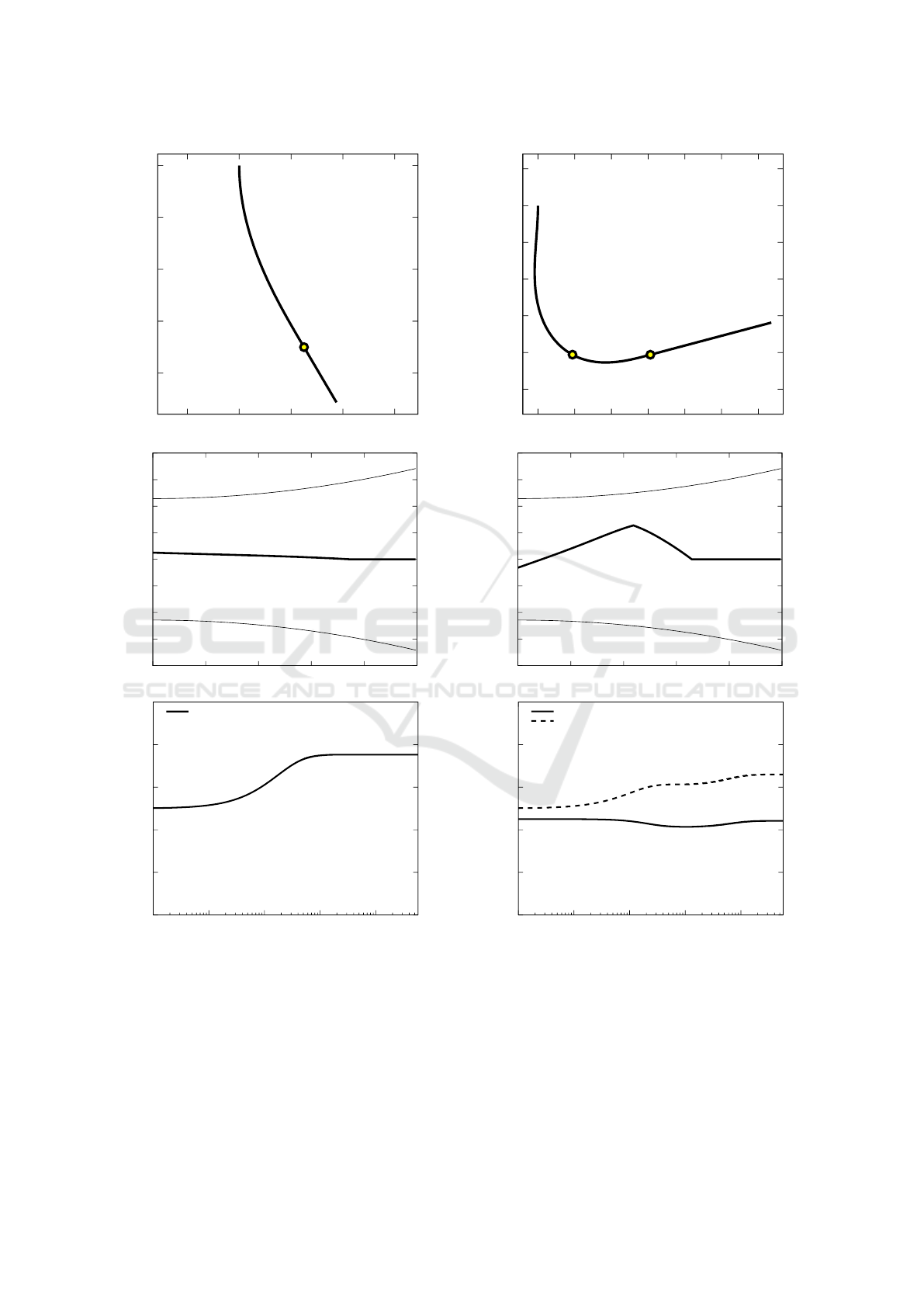
We begin with the simple test of a single target
point p
1
= (0.25,−0.7), Test 1. In Figure 1-(a) we
show the computed optimal configuration q of the
manipulator, the target point (black circle) and the
optimal contact point (yellow circle), while Figure
1-(b) represents the corresponding signed curvature
(thicker line) as a function of s ∈ [0,1], and the thresh-
olds ±
¯
ω(s) (thin lines). Finally, in Figure 1-(c) we
show the behavior of the contact value s
1
∈ I
γ
versus
the total number of iterations to reach convergence,
i.e. accounting for both inner and outer loops in Al-
gorithm 1. We clearly observe the sliding of s
1
toward
the free end, and its convergence.
In Test 2, we choose the two target points p
1
=
(0.094,−0.406), p
2
= (0.306, −0.406), and we re-
port the results in Figure 2. In particular, we observe
the evolution of the contact values s
1
and s
2
in Fig-
ure 2-(c): their behavior is similar to the one of the
previous test for about the first 10
3
iterations. In this
phase the manipulator is attracted and then pinned to
the target points, due to the large value of the penalty
parameter τ
1
. Once the corresponding target term in
L
(k)
is sufficiently reduced, the optimization proceeds
trying to decrease the curvature term. This is done in
the remaining iterations, where we observe a further
sliding of s
1
and s
2
before the convergence.
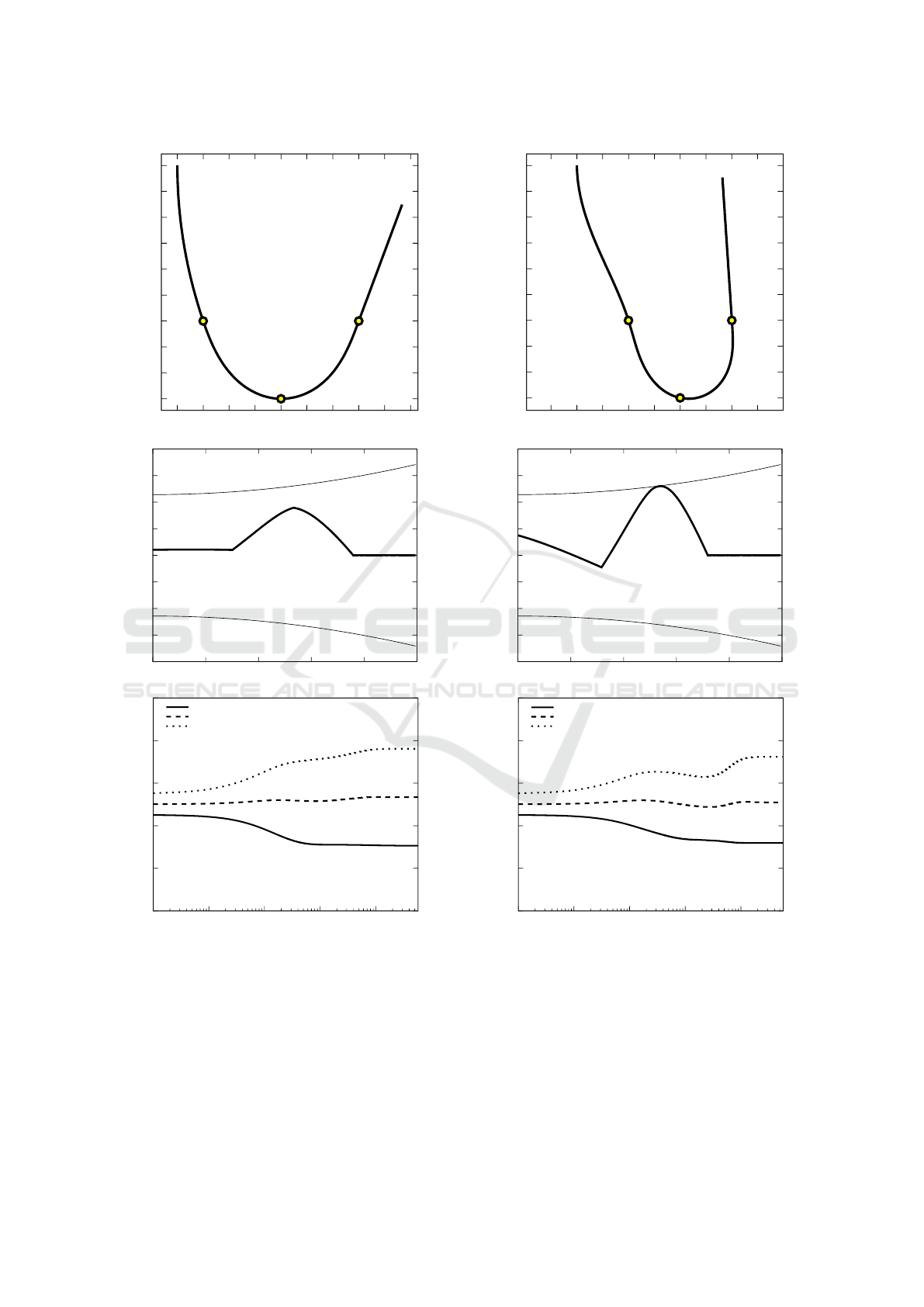
We proceed by considering the case of three tar-
get points at closer and closer distances, that is Test
3, 4 and 5. Figure 3 shows the results for Test 3,
with p
1
= (0.05,−0.3), p
2
= (0.2,−0.45) and p
3
=
(0.35,−0.3), while Figure 4 corresponds to Test 4,
with p
1
= (0.1,−0.3), p
2
= (0.2,−0.45) and p
3
=
(0.3,−0.3). For both configurations, we observe a
behavior of the contact values s
1
,s
2
,s
3
similar to the
previous test, but, in the second one, the final slid-
ing phase is much more evident. This is due to the
closer distance between p
1
and p
3
, forcing the curva-
ture of the manipulator, during the optimization, up
to the threshold
¯
ω on a large interval. Hence, the
optimal solution prefers to retract, adding a double
change of sign in the curvature around p
1
and reach-
ing
¯
ω on a much smaller interval, see Figure 4-(b)
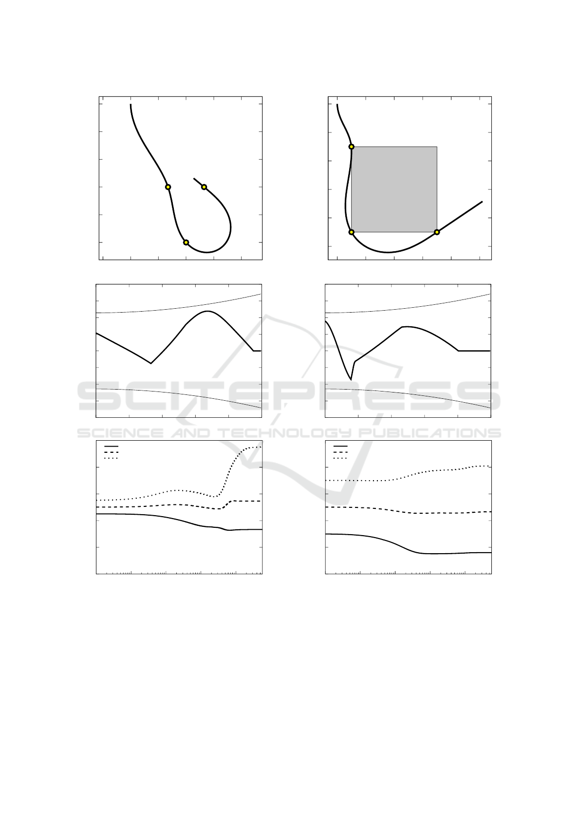
and also Figure 3-(b) for comparison. Finally, Fig-
ure 5 corresponds to Test 5 with p
1
= (0.135, −0.3),
p
2
= (0.2,−0.5) and p
3
= (0.265,−0.3), which pro-
Multi-target Optimal Control Problems for a Tentacle-like Soft Manipulator
43

-0.8
-0.6
-0.4
-0.2
0
-0.2 0 0.2 0.4 0.6
(a)
-20
-15
-10
-5
0
5
10
15
20
0 0.2 0.4 0.6 0.8 1
(b)
0
0.2
0.4
0.6
0.8
1
1 10 100 1000 10000
s
1
(c)
Figure 1: Test 1, optimal configuration (a), optimal cur-
vature (b), and convergence history of the optimal contact
value (c).
vides an even more extreme configuration. Indeed,
the requested bending for touching the target points
is so high that it is better for the manipulator to re-
tract almost up to its free end, as shown by the large
sliding of the contact value s
3
in Figure 5-(c). The op-
-0.5
-0.4
-0.3
-0.2
-0.1
0
0.1
0 0.1 0.2 0.3 0.4 0.5 0.6
(a)
-20
-15
-10
-5
0
5
10
15
20
0 0.2 0.4 0.6 0.8 1
(b)
0
0.2
0.4
0.6
0.8
1
1 10 100 1000 10000
s
1
s
2
(c)
Figure 2: Test 2, optimal configuration (a), optimal curva-
ture (b), and convergence history of the optimal contact val-
ues (c).
timal solution still adds a double change of sign in the
curvature around p
1
, with larger values (in modulus)
in the part preceding p
1
, see also Figure 4 for com-
parison.
We now consider two examples including the square
ICINCO 2021 - 18th International Conference on Informatics in Control, Automation and Robotics
44

-0.45
-0.4
-0.35
-0.3
-0.25
-0.2
-0.15
-0.1
-0.05
0
0 0.05 0.1 0.15 0.2 0.25 0.3 0.35 0.4 0.45
(a)
-20
-15
-10
-5
0
5
10
15
20
0 0.2 0.4 0.6 0.8 1
(b)
s
3
s
1
s
2
0
0.2
0.4
0.6
0.8
1
1 10 100 1000 10000
(c)
Figure 3: Test 3, optimal configuration (a), optimal curva-
ture (b), and convergence history of the optimal contact val-
ues (c).
obstacle described above. In Test 6, we choose
p
1
= (0.05,−0.15), p
2
= (0.05,−0.45) and p
3
=
(0.35,−0.45), namely three vertices of the square,
and we show the results in Figure 6. It is worth not-
ing that the manipulator touches the obstacle just at
-0.45
-0.4
-0.35
-0.3
-0.25
-0.2
-0.15
-0.1
-0.05
0
-0.05 0 0.05 0.1 0.15 0.2 0.25 0.3 0.35
(a)
-20
-15
-10
-5
0
5
10
15
20
0 0.2 0.4 0.6 0.8 1
(b)
s
1
s
2
s
3
0
0.2
0.4
0.6
0.8
1
1 10 100 1000 10000
(c)
Figure 4: Test 4, optimal configuration (a), optimal curva-
ture (b), and convergence history of the optimal contact val-
ues (c).
the target points, but not along the left and bottom
sides. The reason is twofold: first, a flat configuration
across the corner p
2
would produce a jump in the tan-
gent vector q
s
and hence an infinite curvature at p
2
;
second, the first term in the functional (4), namely the
Multi-target Optimal Control Problems for a Tentacle-like Soft Manipulator
45

-0.5
-0.4
-0.3
-0.2
-0.1
0
-0.1 0 0.1 0.2 0.3 0.4
(a)
-20
-15
-10
-5
0
5
10
15
20
0 0.2 0.4 0.6 0.8 1
(b)
s
1
s
2
s
3
0
0.2
0.4
0.6
0.8
1
1 10 100 1000 10000
(c)
Figure 5: Test 5, optimal configuration (a), optimal curva-
ture (b), and convergence history of the optimal contact val-
ues (c).
squared L
2
norm of the weighted curvature, acts as
a regularization. It prevents the curvature to develop
jump singularities (or, in other words, it forbids bang-
bang controls, if we recall that |q
ss
| =
¯
ω|u| by (1)),
and it replaces them with suitable continuous transi-
-0.5
-0.4
-0.3
-0.2
-0.1
0
0 0.1 0.2 0.3 0.4 0.5
(a)
-20
-15
-10
-5
0
5
10
15
20
0 0.2 0.4 0.6 0.8 1
(b)
s
1
s
2
s
3
0
0.2
0.4
0.6
0.8
1
1 10 100 1000 10000
(c)
Figure 6: Test 6, optimal configuration (a), optimal curva-
ture (b), and convergence history of the optimal contact val-
ues (c).
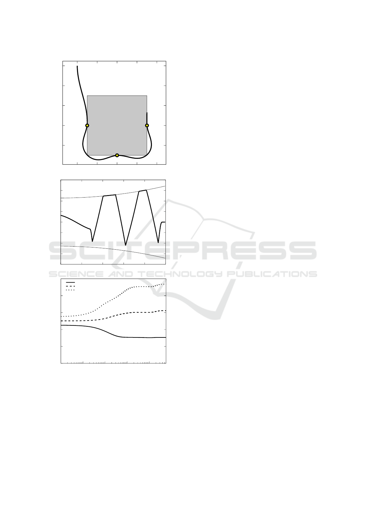
tions. This is more evident in our last and much dif-
ficult experiment, Test 7, shown in Figure 7, where
the target points p
1
= (0.05,−0.3), p
2
= (0.2,−0.45)
and p
3
= (0.35,−0.3) corresponds to the midpoints
of three sides of the square. Note also that, in order to
ICINCO 2021 - 18th International Conference on Informatics in Control, Automation and Robotics
46

-0.4
-0.3
-0.2
-0.1
0
0 0.1 0.2 0.3 0.4
(a)
-20
-15
-10
-5
0
5
10
15
20
0 0.2 0.4 0.6 0.8 1
(b)
s
1
s
2
s
3
0
0.2
0.4
0.6
0.8
1
1 10 100 1000 10000
(c)
Figure 7: Test 7, optimal configuration (a), optimal cur-
vature (b), and convergence history of the optimal contact
points (c).
avoid the bottom corners of the obstacle, the manipu-
lator is forced to push its curvature up to the threshold
¯
ω on two quite large intervals.
5 CONCLUSIONS
The present paper is part of an ongoing investiga-
tion related to the optimal control of tentacle-like pla-
nar manipulators. The model, generalizing the Euler-
Bernoulli beam, is discussed here in the stationary
case. We focused on the problem to find optimal
configurations of the manipulator touching some pre-
scribed points on the boundary of an obstacle, while
minimizing a quadratic cost on the curvature controls.
The numerical tests confirm the consistency and ap-
plicability of our theoretical approach.
We regard at these results as a preliminary step
towards optimal grasping problems. More precisely,
here we addressed the problem to touch a finite set
of fixed target points (while avoiding an obstacle and
optimizing the shape of the manipulator). Our next
step will be to select among the boundary of a tar-
get object, those (four) optimal target points ensuring
planar force closure conditions. The goal of a forth-
coming investigation is indeed to optimize both the
target points as well as the contact sub-region of the
manipulator and the associated controls, in order to
get a steady, optimal grasp of a planar object.
REFERENCES
Bobrow, J. E., Dubowsky, S., and Gibson, J. (1983). On the
optimal control of robotic manipulators with actuator
constraints. In 1983 American Control Conference,
pages 782–787. IEEE.
Cacace, S., Lai, A. C., and Loreti, P. (2019a). Control strate-
gies for an octopus-like soft manipulator. In Proceed-
ings of the 16th International Conference on Informat-
ics in Control, Automation and Robotics - Volume 1:
ICINCO,, pages 82–90. INSTICC, SciTePress.
Cacace, S., Lai, A. C., and Loreti, P. (2019b). Optimal
reachability and grasping for a soft manipulator. In
International Conference on Informatics in Control,
Automation and Robotics, pages 16–34. Springer.
Cacace, S., Lai, A. C., and Loreti, P. (2020a). Modeling and
optimal control of an octopus tentacle. SIAM Journal
on Control and Optimization, 58(1):59–84.
Cacace, S., Lai, A. C., and Loreti, P. (2020b). Opti-
mal reachability with obstacle avoidance for hyper-
redundant and soft manipulators. In ICINCO 2020
- Proceedings of the 17th International Conference
on Informatics in Control, Automation and Robotics,
pages 134–141.
Cacace, S., Lai, A. C., and Loreti, P. (2021). Constrained
reachability problems for a planar manipulator. arXiv
preprint, arXiv:2101.08149.
Christian Kanzow, D. S. and Wachsmuth, D. (2018). An
augmented lagrangian method for optimization prob-
lems in banach spaces. SIAM Journal on Control and
Optimization, 56(1):272 – 291.
Multi-target Optimal Control Problems for a Tentacle-like Soft Manipulator
47

George Thuruthel, T., Ansari, Y., Falotico, E., and Laschi,
C. (2018). Control strategies for soft robotic manipu-
lators: A survey. Soft robotics, 5(2):149–163.
Hestenes, M. (1969). Multiplier and gradient methods.
Journal of Optimization Theory and Applications,
4:303–320.
Hughes, J., Culha, U., Giardina, F., Guenther, F., Rosendo,
A., and Iida, F. (2016). Soft manipulators and grip-
pers: A review. Frontiers in Robotics and AI, 3:69.
Jones, B. A. and Walker, I. D. (2006). Kinematics for mul-
tisection continuum robots. IEEE Transactions on
Robotics, 22(1):43–55.
Kang, R., Kazakidi, A., Guglielmino, E., Branson, D. T.,
Tsakiris, D. P., Ekaterinaris, J. A., and Caldwell,
D. G. (2011). Dynamic model of a hyper-redundant,
octopus-like manipulator for underwater applications.
In Intelligent Robots and Systems (IROS), 2011
IEEE/RSJ International Conference on, pages 4054–
4059. IEEE.
Lai, A. C. and Loreti, P. (2014). Robot’s hand and expan-
sions in non-integer bases. Discrete Mathematics &
Theoretical Computer Science, 16(1).
Lai, A. C., Loreti, P., and Vellucci, P. (2016). A fibonacci
control system with application to hyper-redundant
manipulators. Mathematics of Control, Signals, and
Systems, 28(2):15.
Laschi, C. and Cianchetti, M. (2014). Soft robotics: new
perspectives for robot bodyware and control. Frontiers
in bioengineering and biotechnology, 2:3.
Laschi, C., Cianchetti, M., Mazzolai, B., Margheri, L., Fol-
lador, M., and Dario, P. (2012). Soft robot arm in-
spired by the octopus. Advanced Robotics, 26(7):709–
727.
Michalak, K., Filipiak, P., and Lipinski, P. (2014). Multi-
objective dynamic constrained evolutionary algorithm
for control of a multi-segment articulated manipulator.
In International Conference on Intelligent Data En-
gineering and Automated Learning, pages 199–206.
Springer.
Powell, M. (1969). A method for nonlinear constraints in
minimization problems. Academic Press, New York,
NY.
Rus, D. and Tolley, M. T. (2015). Design, fabrication and
control of soft robots. Nature, 521(7553):467–475.
Wang, B., Wang, J., Zhang, L., Zhang, B., and Li, X.
(2016). Cooperative control of heterogeneous uncer-
tain dynamical networks: An adaptive explicit syn-
chronization framework. IEEE transactions on cyber-
netics, 47(6):1484–1495.
ICINCO 2021 - 18th International Conference on Informatics in Control, Automation and Robotics
48