Deep Learning for RF-based Drone Detection and Identiﬁcation using

Welch’s Method

Mahmoud Almasri

LABSTICC, UMR 6285 CNRS, ENSTA Bretagne, 2 rue F. Verny, 29806 Brest Cedex 9, France

Keywords:

Artiﬁcial Intelligence, Deep Neural Network, Drone Identiﬁcation and Classiﬁcation, Welch.

Abstract:

Radio Frequency (RF) combined with the deep learning methods promised a solution to detect the presence

of the drones. Indeed, the classical techniques (i.e. radar, vision and acoustics, etc.) suffer several drawbacks

such as difﬁcult to detect the small drones, false alarm of ﬂying birds or balloons, the inﬂuence of the wind

on the performance, etc. For an effective drones’s detection, two main stages should be established: Feature

extraction and feature classiﬁcation. The proposed approach in this paper is based on a novel feature extraction

method and an optimized deep neural network (DNN). At ﬁrst, we present a novel method based on Welch

to extract meaningful features from the RF signal of drones. Later on, three optimized Deep Neural Network

(DNN) models are considered to classify the extracted features. The ﬁrst DNN model can be used to detect the

presence of the drones and contains two classes. The second DNN help us to detect and recognize the type of

the drone with 4 classes: A class for each drone and the last one for the RF background activities. In the third

model, 10 classes have been considered: the presence of the drone, its type, and its ﬂight mode (i.e. Stationary,

Hovering, ﬂying with or without video recording). Our proposed approach can achieve an average accuracy

higher than 94% and it signiﬁcantly improves the accuracy, up to 30%, compared to existing methods.

1 INTRODUCTION

Tackling malicious and dangerous Unmanned Aerial

Vehicles (UAVs) use requires the parallel devel-

opment of systems capable of detecting, tracking

and recognizing UAVs in an automatic and non-

collaborative way. Indeed, the development of drones

and the threats for sensitive sites make their detection

and identiﬁcation critical. It is therefore necessary to

develop robust, reliable and inexpensive solutions to

locate and identify these drones. Several modalities

are available to deal with this problem, such as optical

or radar imagery, the detection of Radio-Frequency

(RF) communications or even acoustics. In (Bernar-

dini et al., 2017), acoustic drone localization and de-

tection has been proposed using support vector ma-

chines. In (Chang et al., 2018; Busset et al., 2015), the

authors propose to use the acoustic cameras method-

ology to detect and identify the drones. Video detec-

tion is also possible but quickly limited by the particu-

lar experimental conditions (Ramamonjy et al., 2016).

However, very high performance cameras should be

dedicated to this task, and require an initial localiza-

https://orcid.org/0000-0002-9106-4020

tion step to be able to target the drone beforehand.

In (Bisio et al., 2018), Radar imagery shows limited

performance due to little reﬂected radar signal portion

that mainly depends on the stealth technology.

RF signal emitted from UAVs is recently attracted

more attention to detect malicious drones and is suited

to be used in several scenarios (Azari et al., 2018).

This methodology is nor depends on the used wire-

less technologies of drones such as Wi-Fi, Bluetooth,

4G, etc. RF combined with the Deep Neural Net-

work (DNN) may provide a more effective solution

for drones detection and classiﬁcation. However, the

DNN model is widely suggested in several ﬁelds such

as speech recognition (Chan et al., 2016; Graves et al.,

2013), signal compression (Al-Sa’D et al., 2018), and

in other ﬁelds (LeCun et al., 2015).

The DNN model has emerged as the most impor-

tant and popular Artiﬁcial Intelligence (AI) technique

(Deng et al., 2018; Zhao and Gao, 2019).

In this paper, the two main challenges for drones de-

tection and identiﬁcation are suggested: feature ex-

traction and feature classiﬁcation. The aim of feature

extraction is to get a low dimensional representation

of the data without losing information of the original

data space. Then, the complexity of the data is re-

208

Almasri, M.

Deep Learning for RF-based Drone Detection and Identiﬁcation using Welch’s Method.

DOI: 10.5220/0010530302080214

In Proceedings of the 10th International Conference on Data Science, Technology and Applications (DATA 2021), pages 208-214

ISBN: 978-989-758-521-0

Split Data

Welch’s

Method

Noise

Elimination

Train Data

Test Data

Model Fit

Result Evaluation

Data are divided

into overlapping

segments

Add specified

windows to each

segments

FFT to

windowed

segments

Periodogram of each

windowed segment

is computed

All Periodograms

are averaged to

obtain Welch PSD

Data

Normalization

Figure 1: Flowchart of the entire process.

0 0.5 1 1.5 2 2.5

Time (s)

-3

-1

-0.5

0.5

Amplitude

RF Signal of Bebop

Figure 2: One segment of Bebop RF signal.

duced to a simple representation.

The second challenge, to classify the features vec-

tor gathered from the feature extraction stage in which

the classiﬁcation in this work is performed using the

DNN model. Generally, the classiﬁcation with a low

feature dimension can accelerate the model speed and

limit storage requirements. In this work, three DNN

models are developed:

• To detect the presence of a drone.

• To detect the presence of a drone, and identify its

type.

• To detect the presence of a drone, identify its type,

and ﬁnally determine its ﬂight mode.

2 PROPOSED APPROACH FOR

FEATURE EXTRACTION

In this section, we present our proposed approach to

extract meaningful features, and prepare the dataset

for classiﬁcation using an optimized DNN model. We

use an open access dataset of (Al-Sa’d et al., 2019),

that contains RF signals for three drones: Parrot Be-

bop, Parrot AR, and DJI Phantom 3. In (Al-Sa’d

et al., 2019), the acquisition is performed under differ-

Split Data

Pwelch

Method

Noise

Eimination

Train Data

Test Data

Model Fit

Result Evaluation

Data are divided

into overlapping

segments

Add specified

windows to each

segments

FFT to

windowed

segments

Periodogram of each

windowed segment

is computed

All Periodograms

are averaged to

obtain Welch PSD

Data

Normalization

Figure 3: Welch PSD algorithm.

ent modes: drones are off (i.e. Background activity),

on and connected, hovering, ﬂying with and without

video recording.

Fig. 1 shows a ﬂowchart of the entire proposed ap-

proach. At ﬁrst, all data are split into small segments

(e.g. of 2.5 ms) in order to obtain a large amount of

the data that are required to train and test the DNN

model. Fig. 2 represents a segment of the obtained

signal of Parrot Bebop.

For Fs = 40MHz, the number of samples in Fig.

2 (also in each segment) is 10

sample. In order to ex-

tract the most important features and reduce the num-

ber of samples in each segment, we focus on Welch’s

method.

Indeed, Welch represents one of the most popu-

lar method to calculate the Power Spectral Density

(PSD) for a given signal (Jahromi et al., 2018). Using

Welch’s method, on the one hand, can signiﬁcantly

decrease the number of the features in the dataset; oth-

erwise, the DNN model will be trained for too long

time, and that may cause the model overﬁtting. On

the other hand, it is necessary to discard the noise

segments, that provide a low power; otherwise, the

accuracy will be signiﬁcantly decreased because the

noise segments are used to train and test the DNN

model

. To perform Welch spectral analysis, Fig. 3

shows the different stages of the Welch’s method. Let

us begin to divide a given signal x into N sample:

x[0], x[1], ..., x[N − 1]. Then, all samples are splitted

into K overlapping segments that is considered, in

most cases, equal to 50%. Let M be the length of

each segment, N is the total number of segments, and

S is the number of samples to shift between segments.

Then, we obtain:

In our DNN model, there is a class for the noise (RF back-

ground activities) in order to train the DNN model to dif-

ferentiate the signal of the drone from the noise. Then, if

all classes contain noise segments, the accuracy will be

signiﬁcantly decreased as in the case of (Al-Sa’d et al.,

2019).

Deep Learning for RF-based Drone Detection and Identiﬁcation using Welch’s Method

209

Segment 1: x[0], x[1], . . . ,x[M − 1]

Segment 2: x[S], x[S + 1], ..., x[M + S − 1]

Segment K: x[N − M], x[N − M + 1], ..., x[N − 1]

For each segment k = 1, . . . , K, compute a windowed

Discrete Fourier Transform (DFT) as follows:

( f ) =

∑

x[m]w[m]exp



−

2π f j



(1)

where m = (k − 1)S, . . . , M + (k − 1)S − 1 and w[m]

represents the window function. Then, calculate the

periodogram P

( f ) for each segment as follows:

( f ) =

( f )|

(2)

where W =

∑

[m]. Finally, average the peri-

odogram for each segments to obtain Welch’s PSD:

( f ) =

∑

k=1

( f ) (3)

After splitting the data and applying Welch’s method

on all segments, a threshold γ is established in order

to eliminate all segments with a low PSD

. Tab. 1

represents all segments in each class before and after

eliminate noise segments that have a PSD lower than

the threshold γ. To ﬁnalize the data preparation, all

segments should be normalized in order to make sure

that the different segments take on similar ranges of

values. Then, the necessary time to train the DNN

model is reduced while still providing the most accu-

rate results (Passalis et al., 2019). In (Sola and Sevilla,

1997), the authors show that the best normalization

method can be achieved when all segments are in the

same magnitude, and specially if they are in the or-

der of one. For this reason, after noise elimination, all

segments are normalized using the min-max method

that provides better results in most object classiﬁca-

tion (Al Shalabi et al., 2006; Saranya and Manikan-

dan, 2013):

x =

x − min(x)

max(x) − min(x)

(4)

After performing Welch’s method and the seg-

ment normalization on the signal of the Bebop in Fig.

2, we obtain Fig. 4.

This threshold level can be chosen with respect to the RF

background activities where there is no-drone signal.

2400 2420 2440 2460 2480

Frequency (MHz)

-150

-100

-50

Pwelch of Bebop for one segment

Figure 4: Welch based estimates, Hamming window, 2050

samples long segment, 50% overlap, min-max normaliza-

tion.

3 DEEP NEURAL NETWORK

MODEL

Deep Neural Network (DNN) has shown surpass-

ing results in various cognitive tasks such as speech

recognition, object detection and identiﬁcation, etc.

At ﬁrst, we present the DNN concept and general ar-

chitecture. Later on, we optimize the architecture of

the DNN model in order to accelerate the training

time and also to achieve a better accuracy. A DNN

model has an input layer, hidden layers and an out-

put layer. For a given DNN model, the mathemati-

cal input-output relationship can be expressed as fol-

lows(He and Xu, 2010):

= f

(l−1)

+ b

), (5)

(l)







(l)

·· · w

(l)

(l−1)

(l)

·· · w

(l)

(l−1)

(l)

·· · w

(l)

(l−1)







(6)

is the output of layer l and the input to layer

l + 1 for the k

segment; z

(l−1)

represents the out-

put of layer (l − 1) and the input to layer l; for in-

stance, z

stands for the k

segment at the input layer

and z

represents the classiﬁcation vector for the k

segment where L is the output layer; f

is the acti-

vation function of layer l; This later can be any lin-

ear or non-linear function, such as: the rectiﬁed linear

unit (ReLU), Sigmoid, Softmax, TanH, etc. W

is the

weight matrix of layer l; w

is the weight between

the p

neuron of layer l and the q

neuron of layer

l −1; b

= [b

, b

, . . . , b

)

] is the bias vector of layer

DATA 2021 - 10th International Conference on Data Science, Technology and Applications

210

Table 1: Class Labels, Acronyms, and Class Sample Rate before and after the Preprocessing.

Classes Class Name Acronyms nb. of segments before nb. of segments after

the preprocessing the preprocessing

1 No-Drone (Background activities) ND 4100 4100

2 Bebop Static BS 2100 832

3 Bebop Hovering BH 2100 695

4 Bebop Flying BF 2100 720

5 Bebop Flying & Video recording BFV 2100 696

6 AR Static AS 2100 659

7 AR Hovering AH 2100 526

8 AR Flying AF 2100 566

9 AR Flying & Video recording AFV 1800 886

10 Phantom Static PS 2100 1627

l; H

is the total number of neurons in layer l; for in-

stance, H

is the number of features at the input and

is the number of classes in the classiﬁcation vector

at the output.

3.1 DNN Model Optimization

In a DNN model, the weight and biases are updated

through a supervised learning process with respect

to minimizing the classiﬁcation error (Bottou, 2010).

Several classiﬁcation loss functions are adapted to

DNN models and widely used in the literature, such as

Mean Square Error (MSE), cross-entropy, etc. Cross-

entropy is the most commonly used loss function for

multi-class classiﬁcation problems (Nielsen, 2015),

(Zhu et al., 2020) and (Nasr et al., 2002). Cross-

entropy for a multi-class classiﬁcation task measures

the dissimilarity between the target label distribution

and the predicted one ˆy

, and can be expressed as

follows:

L(y

, ˆy

) = −

∑

j=1

log( ˆy

) (7)

In eq. (7), the Cross-entropy is conﬁgured with C

class (C = H

), and a ‘Softmax‘ activation function

should be used at the output layer in order to pre-

dict the probability for each class (Liu et al., 2016;

Kobayashi, 2019; Agarwala et al., 2020). While for

hidden layers, we use the rectiﬁed linear unit (ReLU)

that represents the most used activation function by

default for performing a majority of the deep learning

tasks. Softmax and ReLU functions are respectively

expressed in eq. (8) and (9):

f (x

) =

∑

j=1

, for i=1,...,C (8)

f (x

) =

(

> 0

0 x

≤ 0

(9)

Let’s start to determine the best number of layers

and neurons in the hidden layers. For the input layer,

the number of neurons is equal to 2050 that repre-

sents the number of samples in each segment. While

the number of neurons at the output is equal to 2, 4 or

10 classes for the ﬁrst, second, and third DNN model.

For hidden layers, until now, there were no-deﬁnitive

rules for choosing the number of hidden layers, and

the best number of neurons in each hidden layer. Sev-

eral methods are used without providing an exact for-

mula for determining the number of hidden layers as

well as the number of neurons in each hidden layer.

For the number of hidden layers, the best hidden lay-

ers is achieved when the number of layers ranges from

1-5 (Ariﬁn et al., 2019). However, adding more un-

necessary hidden layer can signiﬁcantly increase the

complexity of the network.

For the number of neurons in hidden layers, several

works attempt different methods trying to maximize

the model accuracy, and some rules are suggested:

• The required hidden neurons are

(or from 70%

to 90%) of the size of the input layer (Boger and

Guterman, 1997).

• The number of hidden neurons should be less than

twice of the number of neurons in the input layer

(Berry and Linoff, 2004).

• The number of hidden neurons can be as high as

the number of training segments (Huang, 2003).

• The number of hidden neurons should be between

the input layer neurons and the output layer ones

(Blum, 1992).

Based on the above discussion, and to reduce the com-

plexity of the DNN model, we consider three layers

with the following number of neurons: 256, 128 and

64.

Deep Learning for RF-based Drone Detection and Identiﬁcation using Welch’s Method

211

Fold 1

Fold 2

Fold 10

𝐷

𝑣𝑎𝑙,1

𝐷

𝑡𝑟𝑎𝑖𝑛,1

Figure 5: 10-fold cross-validation. The data is randomly

partitioned into 10 blocks, each of them contains 10% of the

data. 90% of the data are used to train the model training

and 10% for model validation.

3.2 K-fold Cross-Validation

K-fold Cross-Validation represents one of the most

used technique for model evaluation in machine learn-

ing practice. However, machine learning models

sometimes cannot generalize well on unseen data that

has not been trained yet. To ensure that the model is

relevant and can perform well on new data, K-fold

Cross-Validation is recommended. As well, it en-

sures that all RF segments in the dataset has the same

chance to be in training and test set. In K-fold Cross-

Validation, RF segments are divided into K blocks

with equal size. Then, one block is used for the vali-

dation while the other K −1 blocks contribute to train

the DNN model, and a validation performance can

be calculated. The operation is repeated K times, by

selecting another validation block, in order to obtain

a model that have both low bias and variance. The

global cross-validated performance can be obtained

by averaging the K performance measurements.

Fig. 5 illustrates the K-fold cross validation for

K = 10 where D

val,1

in the ﬁrst fold represents the

data validation and blocks D

train,1

serve as training

data. In (Raschka, 2018), the experiments show that

K = 10 represents a good choice for K.

4 RESULTS AND DISCUSSION

In this section, we use several metrics in order to eval-

uate the performance of our proposed method: Ac-

curacy, Precision, recall, error, false discovery rate

(FDR), false negative rate (FNR) and F1 scores via

confusion matrices. These metrics are deﬁned as fol-

lows:

Accuracy =

T P + T N

T P + T N + FP + FN

(10)

Precision =

T P

T P + FP

(11)

Recall =

T P

T P + FN

(12)

Error = 1 −Accuracy (13)

FDR = 1 −Precision (14)

FNR = 1 −Recall (15)

where T P, T N, FP and FN are true positives, true

negatives, false positives and false negatives respec-

tively. We develop three DNNs models for drones

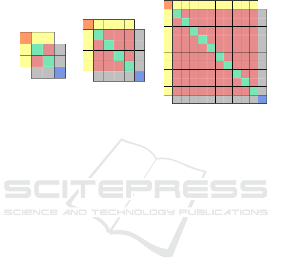
detection and identiﬁcation. The Confusion Matrix

of the three DNN models for 2-class, 4-class and 10-

class are respectively shown in Figs. 6a, 6b and 6c.

In that ﬁgures, the rows of the inner 2x2, 4x4 and

10x10 matrices represent the predicted class while the

columns correspond to the true class. The diagonal

cells, exhibited in green, represent the number of seg-

ments that are correctly classiﬁed, while the red cells

refer to the incorrectly classiﬁed segments. As well

as, each cell show the number of segments and the

percentage of the total number of segments. The gray

cells in the right column show the precision and FDR

in green and red respectively. Furthermore, the gray

cells in the row at the bottom illustrate the recall in

green, and FNR in red. In addition, the blue cell in the

bottom right of the plot shows the overall accuracy in

green, and the error in red. Moreover, the yellow col-

umn and row on the far left and top show the F1 scores

for predicting each class in green and its complemen-

tary in red, (1-F1 score), for completeness. Finally,

the orange cell in the upper left of the plot shows the

averaged F1 score for all classes in green and its com-

plementary in red. The ﬁrst DNN model in Fig. 6a,

for two classes, shows that the average accuracy is

about of 99.7%, average error of 0.3% and average F1

score of 99.7%. Fig. 6b depicts the classiﬁcation per-

formance of the second DNN model, which detects

the presence of a drone and identiﬁes its type. Results

demonstrate an average accuracy of 97.7%, average

error of 2.3%, and average F1 score of 97.5%.

We should notice that the average accuracy is

signiﬁcantly improved using our approach based on

Welch’s method compared to the proposed methods in

(Al-Sa’d et al., 2019; Al-Emadi and Al-Senaid, 2020;

Allahham et al., 2020). Indeed, the achieved accura-

cies in the latter references, for 4 classes, are respec-

tively: 84.5%, 85.8 % and 94.6 %.

Finally, Fig. 6c illustrates the classiﬁcation per-

formance of the third DNN model which detects the

presence of a drone, identiﬁes its type, and determines

its ﬂight mode. Results demonstrate an average accu-

racy of 94.5%, average error of 5.5%, and average

DATA 2021 - 10th International Conference on Data Science, Technology and Applications

212

No-Drone Drone

Target Class

No-Drone

Drone

Output Class

4082

36.1%

0.2%

99.6%

0.4%

0.1%

7191

63.6%

99.8%

0.2%

99.6%

0.4%

99.8%

0.2%

99.7%

0.3%

99.6%

0.4%

99.8%

0.2%

99.6%

0.4%

99.8%

0.2%

99.7%

0.3%

(a) Confusion Matrix of the

ﬁrst DNN model

ND B A P

Target Class

Output Class

4084

36.1%

0.1%

0.0%

99.6%

0.4%

0.1%

2859

25.3%

0.6%

0.1%

97.1%

2.9%

0.0%

107

0.9%

2523

22.3%

0.0%

95.7%

4.3%

0.0%

0.2%

1585

14.0%

97.4%

2.6%

99.7%

0.3%

95.4%

4.6%

96.5%

3.5%

99.1%

0.9%

97.7%

2.3%

99.6%

0.4%

96.2%

3.8%

96.1%

3.9%

98.2%

1.8%

99.6%

0.4%

96.2%

3.8%

96.1%

3.9%

98.2%

1.8%

97.5%

2.5%

(b) Confusion Matrix of the second

DNN model

ND BS BH BF BFV AS AH AF AFV PS

Target Class

BFV

AFV

Output Class

4085

36.1%

0.0%

99.6%

0.4%

0.0%

786

7.0%

0.1%

0.0%

0.2%

0.0%

94.5%

5.5%

0.0%

650

5.7%

0.1%

0.0%

0.1%

0.2%

0.1%

0.0%

93.5%

6.5%

0.0%

647

5.7%

0.2%

0.0%

0.1%

0.0%

89.9%

10.1%

0.0%

0.1%

0.2%

654

5.8%

0.0%

94.0%

6.0%

0.0%

0.1%

0.0%

604

5.3%

0.1%

0.0%

91.7%

8.3%

0.0%

0.1%

0.0%

0.2%

409

3.6%

0.5%

0.2%

0.0%

77.8%

22.2%

0.0%

0.1%

0.0%

0.1%

0.4%

470

4.2%

0.2%

0.0%

83.0%

17.0%

0.0%

0.2%

0.4%

793

7.0%

0.0%

89.5%

10.5%

0.0%

0.1%

0.0%

0.1%

0.0%

1585

14.0%

97.4%

2.6%

99.7%

0.3%

96.6%

3.4%

92.7%

7.3%

91.4%

8.6%

94.9%

5.1%

87.4%

12.6%

76.3%

23.7%

75.9%

24.1%

93.2%

6.8%

99.0%

1.0%

94.5%

5.5%

99.6%

0.4%

95.5%

4.5%

93.1%

6.9%

90.6%

9.4%

94.4%

5.6%

89.5%

10.5%

77.0%

23.0%

79.3%

20.7%

91.3%

8.7%

98.2%

1.8%

99.6%

0.4%

95.5%

4.5%

93.1%

6.9%

90.6%

9.4%

94.4%

5.6%

89.5%

10.5%

77.0%

23.0%

79.3%

20.7%

91.3%

8.7%

98.2%

1.8%

90.8%

9.2%

Figure 6: Confusion matrix of the three DNN models. Fig. 6a represents two classes: No-Drone and Drone. Fig. 6b depicts the

performance of the second DNN model for 4 classes: ND (No-drone), B (Bebop), A (AR) and P (Phantom). The Acronyms

in Fig. 6c are shown in Tab. 1.

F1 score of 90.8%. While, the obtained accuracies

in (Al-Sa’d et al., 2019; Al-Emadi and Al-Senaid,

2020; Allahham et al., 2020) are respectively: 46.8%,

59.2% and 87.4%. Then, the average accuracy of our

proposed method, for 10 classes, can be greatly en-

hanced by 47%, 35% and 7% compared to the pro-

posed methods in the latter references.

5 CONCLUSION

In Intelligent detection and identiﬁcation techniques

have emerged vastly by the rise of data driven algo-

rithms, such as neural networks. In the Deep Neural

Network (DNN), extracting features from given data

represents a critical importance for the successful ap-

plication of machine learning. In this work, we pro-

posed a novel approach based on Welch’s method for

feature extraction in order to enhance the classiﬁca-

tion performance of multi-class and maximize the av-

erage accuracy. Using Welch’s method, the number

of extracted features at the input of the DNN model

can be reduced. Moreover, it can estimate if a given

segment of data contains an useful information or not,

so that the noise segments can be eliminated. Three

DNN models have been used to classify the extracted

features, and then detect the presence of a drone, iden-

tify its type and ﬁnally determine its ﬂight mode. In

the ﬁrst DNN model, for two classes, the achieved

average accuracy is about of 99.7%. By increasing

the number of classes in the second DNN model, 4

classes are used, the average accuracy is slightly de-

creased to 97.7%. In the last DNN model with 10

classes, the obtained accuracy is about of 94.5% that

is enhanced up to 47% compared to existing methods.

In the future work, another important feature ex-

traction methods can be used in the frequency or time

domains, such as Entropy, Skewness, kurtosis, etc.

Another potential research direction is to apply an-

other powerful machine learning technologies to ad-

dress the fundamental visual feature extraction issue.

REFERENCES

Agarwala, A., Pennington, J., Dauphin, Y., and Schoen-

holz, S. (2020). Temperature check: theory and prac-

tice for training models with softmax-cross-entropy

losses. arXiv preprint arXiv:2010.07344.

Al-Emadi, S. and Al-Senaid, F. (Doha, Qatar, February,

2020). Drone detection approach based on radio-

frequency using convolutional neural network. In

IEEE International Conference on Informatics, IoT,

and Enabling Technologies, pages 29–34.

Al-Sa’d, M. F., Al-Ali, A., Mohamed, A., Khattab, T., and

Erbad, A. (2019). Rf-based drone detection and iden-

tiﬁcation using deep learning approaches: An initia-

tive towards a large open source drone database. Fu-

ture Generation Computer Systems, 100:86–97.

Al-Sa’D, M. F., Tlili, M., Abdellatif, A. A., Mohamed,

A., Elfouly, T., Harras, K., O’Connor, M. D., et al.

(2018). A deep learning approach for vital signs com-

pression and energy efﬁcient delivery in mhealth sys-

tems. IEEE Access, 6:33727–33739.

Al Shalabi, L., Shaaban, Z., and Kasasbeh, B. (2006). Data

mining: A preprocessing engine. Journal of Computer

Science, 2(9):735–739.

Allahham, M. S., Khattab, T., and Mohamed, A. (Doha,

Deep Learning for RF-based Drone Detection and Identiﬁcation using Welch’s Method

213

Qatar, February, 2020). Deep learning for rf-based

drone detection and identiﬁcation: A multi-channel 1-

d convolutional neural networks approach. In IEEE

International Conference on Informatics, IoT, and En-

abling Technologies, pages 112–117.

Ariﬁn, F., Robbani, H., Annisa, T., and Ma’arof, N. (2019).

Variations in the number of layers and the number of

neurons in artiﬁcial neural networks: Case study of

pattern recognition. In Journal of Physics: Confer-

ence Series, volume 1413, page 012016.

Azari, M. M., Sallouha, H., Chiumento, A., Rajendran, S.,

Vinogradov, E., and Pollin, S. (2018). Key technolo-

gies and system trade-offs for detection and localiza-

tion of amateur drones. IEEE Communications Mag-

azine, 56(1):51–57.

Bernardini, A., Mangiatordi, F., Pallotti, E., and Capodi-

ferro, L. (2017). Drone detection by acoustic signature

identiﬁcation. Electronic Imaging, 2017(10):60–64.

Berry, M. J. and Linoff, G. S. (2004). Data mining tech-

niques: for marketing, sales, and customer relation-

ship management. John Wiley & Sons.

Bisio, I., Garibotto, C., Lavagetto, F., Sciarrone, A., and

Zappatore, S. (2018). Blind detection: Advanced

techniques for wiﬁ-based drone surveillance. IEEE

Transactions on Vehicular Technology, 68(1):938–

946.

Blum, A. (1992). Neural networks in C++: an object-

oriented framework for building connectionist sys-

tems. John Wiley & Sons, Inc.

Boger, Z. and Guterman, H. (Orlando, FL, USA, October,

1997). Knowledge extraction from artiﬁcial neural

network models. In IEEE International Conference

on Systems, Man, and Cybernetics, Computational

Cybernetics and Simulation, volume 4, pages 3030–

3035.

Bottou, L. (Paris France, August, 2010). Large-scale ma-

chine learning with stochastic gradient descent. In In-

ternational Conference on Computational Statistics.

Busset, J., Perrodin, F., Wellig, P., Ott, B., Heutschi, K.,

uhl, T., and Nussbaumer, T. (2015). Detection and

tracking of drones using advanced acoustic cameras.

In Unmanned/Unattended Sensors and Sensor Net-

works XI; and Advanced Free-Space Optical Commu-

nication Techniques and Applications, volume 9647,

page 96470.

Chan, W., Jaitly, N., Le, Q., and Vinyals, O. (Shanghai,

China, March, 2016). Listen, attend and spell: A

neural network for large vocabulary conversational

speech recognition. In IEEE International Conference

on Acoustics, Speech and Signal Processing.

Chang, X., Yang, C., Wu, J., Shi, X., and Shi, Z. (Shefﬁeld,

UK, July, 2018). A surveillance system for drone

localization and tracking using acoustic arrays. In

IEEE Sensor Array and Multichannel Signal Process-

ing Workshop (SAM).

Deng, C., Liao, S., Xie, Y., Parhi, K. K., Qian, X., and Yuan,

B. (Fukuoka, Japan, October, 2018). Permdnn: Efﬁ-

cient compressed dnn architecture with permuted di-

agonal matrices. In Annual IEEE/ACM International

Symposium on Microarchitecture (MICRO).

Graves, A., Abdelrahman, M., and Hinton, G. (Vancouver,

Canada, 2013). Speech recognition with deep recur-

rent neural networks.

He, X. and Xu, S. (2010). Artiﬁcial neural networks. Pro-

cess neural networks: theory and applications, pages

20–42.

Huang, G.-B. (2003). Learning capability and storage

capacity of two-hidden-layer feedforward networks.

IEEE Transactions on Neural Networks, 14(2):274–

281.

Jahromi, M. G., Parsaei, H., Zamani, A., and Stashuk, D. W.

(2018). Cross comparison of motor unit potential fea-

tures used in emg signal decomposition. IEEE Trans-

actions on Neural Systems and Rehabilitation Engi-

neering, 26(5):1017–1025.

Kobayashi, T. (Cardiff, UK, September, 2019). Large mar-

gin in softmax cross-entropy loss. In British Machine

Vision Conference.

LeCun, Y., Bengio, Y., and Hinton, G. (2015). Deep learn-

ing. nature, 521(7553):436–444.

Liu, W., Wen, Y., Yu, Z., and Yang, M. (New York City,

USA, June, 2016). Large-margin softmax loss for con-

volutional neural networks. In International Confer-

ence on Machine Learning.

Nasr, G. E., Badr, E., and Joun, C. (2002). Cross entropy er-

ror function in neural networks: Forecasting gasoline

demand. In FLAIRS conference, pages 381–384.

Nielsen, M. A. (2015). Neural networks and deep learn-

ing, volume 2018. Determination press San Francisco,

CA.

Passalis, N., Tefas, A., Kanniainen, J., Gabbouj, M., and

Iosiﬁdis, A. (2019). Deep adaptive input normaliza-

tion for time series forecasting. IEEE Transactions on

Neural Networks and Learning Systems.

Ramamonjy, A., Bavu, E., Garcia, A., and Hengy, S. (Le

Mans, France, 2016). D

etection, classiﬁcation et

suivi de trajectoire de sources acoustiques par capta-

tion pression-vitesse sur capteurs mems num

eriques.

In Congr

es de la Soci

e Franc¸aise d’Acoustique-

CFA16/VISHNO.

Raschka, S. (2018). Model evaluation, model selection,

and algorithm selection in machine learning. arXiv

preprint arXiv:1811.12808.

Saranya, C. and Manikandan, G. (2013). A study on

normalization techniques for privacy preserving data

mining. International Journal of Engineering and

Technology, 5(3):2701–2704.

Sola, J. and Sevilla, J. (1997). Importance of input data

normalization for the application of neural networks

to complex industrial problems. IEEE Transactions

on nuclear science, 44(3):1464–1468.

Zhao, C. and Gao, X.-S. (2019). Qdnn: Dnn with

quantum neural network layers. arXiv preprint

arXiv:1912.12660.

Zhu, Q., He, Z., Zhang, T., and Cui, W. (2020). Improv-

ing classiﬁcation performance of softmax loss func-

tion based on scalable batch-normalization. Applied

Sciences, 10(8):2950.

DATA 2021 - 10th International Conference on Data Science, Technology and Applications

214