Uniformly Regular Triangulations for Parameterizing Lyapunov
Functions
Peter Giesl
1 a
and Sigurdur Hafstein
2 b
1
Department of Mathematics, University of Sussex, Falmer, BN1 9QH, U.K.
2
Science Institute, University of Iceland, Dunhagi 3, 107 Reykjav
´
ık, Iceland
Keywords:
Triangulation, Lyapunov Function, CPA Algorithm, Linear Programming.
Abstract:
The computation of Lyapunov functions to determine the basins of attraction of equilibria in dynamical sys-
tems can be achieved using linear programming. In particular, we consider a CPA (continuous piecewise
affine) Lyapunov function, which can be fully described by its values at the vertices of a given triangulation.
The method is guaranteed to find a CPA Lyapunov function, if a sequence of finer and finer triangulations
with a bound on their degeneracy is considered. Hence, the notion of (h,d)-bounded triangulations was intro-
duced, where h is a bound on the diameter of each simplex and d a bound on the degeneracy, expressed by
the so-called shape-matrices of the simplices. However, the shape-matrix, and thus the degeneracy, depends
on the ordering of the vertices in each simplex. In this paper, we first remove the rather unnatural dependency
of the degeneracy on the ordering of the vertices and show that an (h,d)-bounded triangulation, of which the
ordering of the vertices is changed, is still (h,d
∗
)-bounded, where d
∗
is a function of d, h, and the dimension of
the system. Furthermore, we express the degeneracy in terms of the condition number, which is a well-studied
quantity.
1 INTRODUCTION
Lyapunov stability theory is of essential importance
in dynamical systems and control theory and is stud-
ied in practically all textbooks and monographs on
linear and nonlinear systems, cf. e.g. (Zubov, 1964;
Yoshizawa, 1966; Hahn, 1967) or (Sastry, 1999;
Vidyasagar, 2002; Khalil, 2002) for a more modern
treatment. The canonical candidate for a Lyapunov
function for a physical system is its (free) energy.
In particular, a dissipative physical system must ap-
proach the state of a local minimum of the energy.
For general dynamical systems, however, there
is no analytical method to obtain a Lyapunov func-
tion. For this reason, various methods for the numer-
ical generation of Lyapunov functions have emerged.
To name a few, in (Vannelli and Vidyasagar, 1985;
Valmorbida and Anderson, 2017) the numerical gen-
eration of rational Lyapunov functions was studied,
in (Parrilo, 2000; Chesi, 2011; Anderson and Pa-
pachristodoulou, 2015) sum-of-squared (SOS) poly-
nomial Lyapunov functions were parameterized us-
ing semi-definite optimization, see also (Ratschan and
a
https://orcid.org/0000-0003-1421-6980
b
https://orcid.org/0000-0003-0073-2765
She, 2010; Kamyar and Peet, 2015) for other ap-
proaches using polynomials, and in (Giesl, 2007) a
Zubov type PDE was approximately solved using col-
location. For more numerical approaches cf. the re-
view (Giesl and Hafstein, 2015b).
In (Julian et al., 1999; Marin
´
osson, 2002) linear
programming was used to parameterize continuous
and piecewise affine (CPA) Lyapunov functions. In
this approach, a subset of the state space is first tri-
angulated, i.e. subdivided into simplices, and then a
number of constraints are derived for a given nonlin-
ear system, such that a feasible solution to the re-
sulting linear programming problem allows for the
parametrization of a CPA Lyapunov function for the
system.
In (Hafstein, 2004; Hafstein, 2005; Giesl and Haf-
stein, 2014) it was proved that this approach always
succeeds in computing a Lyapunov function for a gen-
eral nonlinear system with an exponentially stable
equilibrium, if the simplices are sufficiently small and
non-degenerate. The proof of this fact used the con-
cept of (h,d)-bounded triangulations, see Definition
3.1, where h > 0 is an upper bound on the diame-
ters of the simplices and d > 0 quantifies the degen-
eracy of the simplices. For the definition of (h,d)-
Giesl, P. and Hafstein, S.
Uniformly Regular Triangulations for Parameterizing Lyapunov Functions.
DOI: 10.5220/0010522405490557
In Proceedings of the 18th International Conference on Informatics in Control, Automation and Robotics (ICINCO 2021), pages 549-557
ISBN: 978-989-758-522-7
Copyright
c
 2021 by SCITEPRESS – Science and Technology Publications, Lda. All rights reserved
549

bounded triangulations one must consider triangula-
tions, of which the order of the vertices of each sim-
plex has been fixed.
The first main contribution of this paper is to show
that if T is an (h,d)-bounded triangulation in R
n
,
n ≥ 2, then any triangulation consisting of the same
simplices as T , but with a different ordering of the
vertices, is an (h,d
∗
)-bounded triangulation with
d
∗
= d(1 + d
√
n −1).
Thus, the property that a triangulation is (h, d)-
bounded depends essentially on the simplices of the
triangulation T , and not the ordering of the vertices of
the simplices. Note that the case n = 1 is trivial and
any ordering of the vertices gives an (h, d)-bounded
triangulation of the line.
The second main contribution is a characteriza-
tion of (h, d)-bounded triangulations using the con-
dition number of the shape-matrices of the simplices,
cf. Definition 4.2. The advantage of this characteri-
zation is that the condition number of a matrix is a
more familiar concept than the degeneracy as defined
in Definition 3.1.
The paper is organized as follows. After intro-
ducing some notations, we define triangulations, CPA
functions, shape-matrices of simplices, and (h, d)-
bounded triangulations in Section 2. In Section 3
we outline the algorithm to compute CPA Lyapunov
functions and explain the relevance of (h,d)-bounded
triangulations for the algorithm. In Section 4 we
prove our main results in Proposition 4.1, 4.4 and 4.5,
before we give conclusions in Section 5.
1.1 Prerequisites and Notation
N
0
denotes the set {0,1,2,. ..,}. For a vector x ∈ R
n
and p ≥1 we define the norm kxk
p
= (
∑
n
i=1
|x
i
|
p
)
1/p
.
We also define kxk
∞
= max
i∈{1,...,n}
|x
i
|. We will re-
peatedly use the norm equivalence relation
kxk
p
≤ kxk
q
≤ n
q
−1
−p
−1
kxk
p
for p > q.
The induced matrix norm k·k
p
is defined by kAk
p
=
max
kxk
p
=1
kAxk
p
. Clearly kAxk
p
≤ kAk
p
kxk
p
. For
a matrix A we write A
T
for its transpose. Recall that
kAk
1
= kA
T
k
∞
= max
i
ka
i
k
1
, where a
i
are the column
vectors of A, and the norm equivalences
1
√
n
kAk
p
≤ kAk
2
≤
√
nkAk
p
for A ∈ R
n×n
and p ∈ {1,∞}. The condition number
κ
p
of a nonsingular matrix A ∈ R
n×n
with respect to
the norm k·k
p
is defined as κ
p
(A) := kAk
p
kA
−1
k
p
.
We utilize a bold-face font for (column) vectors,
e.g. x ∈ R
n×1
= R
n
. For a vector x we write x
i
or [x]
i
for its ith component. We denote by e
1
,e
2
,. ..,e
n
the
standard orthonormal basis of R
n
and by I the identity
matrix. We denote the interior of a set S ⊂ R
n
by S
◦
and its closure by S .
If B ∈ R
n×n
and u,v ∈R
n
, then
uv
T
Buv
T
B = (v
T
Bu)uv
T
B
because v
T
Bu ∈ R. From this simple observation the
very useful Sherman-Morrison lemma on the rank 1
correction A + uv
T
of an invertible matrix A follows,
cf. (Sherman and Morrison, 1950).
Lemma 1.1 (Sherman-Morrison). Let A ∈ R
n×n
be
invertible and u,v ∈R
n
. Then

A + uv
T

−1
= A
−1
−
A
−1
uv
T
A
−1
1 + v
T
A
−1
u
,
provided 1 + v
T
A
−1
u 6= 0. Furthermore, we have the
following identity:
det

A + uv
T

=

1 + v
T
A
−1
u

detA.
The determinant identity can be seen from
(I + xv
T
)x = (1 + v
T
x)x
and
(I + xv
T
)z = z for z ∈ R
n
with v
T
z = 0.
Thus, the eigenvalues of (I + xv
T
) are 1 + v
T
x and
(n −1)-times 1, we have det(I + xv
T
) = 1 + v
T
x, and
it follows with x = A
−1
u that
det

A + uv
T

= det A ·det

I + A
−1
uv
T

=

1 + v
T
A
−1
u

detA.
2 TRIANGULATIONS AND CPA
FUNCTIONS
In this section we will introduce triangulations and
CPA functions as well as the definition of (h, d)-
bounded triangulations.
Definition 2.1. We define the following :
i) The convex-combination of vectors
x
0
,x
1
,. ..,x
m
∈ R
n
, denoted
co{x
0
,x
1
,. ..,x
m
},
is the set of all sums
m
∑
i=0
λ
i
x
i
, where
m
∑
i=0
λ
i
= 1
and ∀i : 0 ≤λ
i
≤ 1.
ICINCO 2021 - 18th International Conference on Informatics in Control, Automation and Robotics
550

ii) The vectors x
0
,x
1
,. ..,x
m
∈ R
n
are said to be
affinely-independent if
m
∑
i=0
λ
i
x
i
= 0 and
m
∑
i=0
λ
i
= 0
implies λ
0
= λ
1
= ··· = λ
m
= 0.
iii) If x
0
,x
1
,. ..,x
m
∈ R
n
are affinely-independent,
then the set S = co{x
0
,x
1
,. ..,x
m
} is called an
m-simplex. The vectors x
0
,x
1
,. ..,x
m
are called
the vertices of S. The set of vertices for
an m-simplex is sometimes denoted by veS =
{x
0
,x
1
,. ..,x
m
}. In R
n
an n-simplex is often re-
ferred to as just a simplex.
iv) For an m-simplex S, define its diameter as:
diam(S) := max
x,y∈S
kx −yk
2
.
We now define a triangulation. For our purposes it
is advantageous to have the order of the vertices of ev-
ery simplex in the triangulation fixed, similar to (Giesl
and Hafstein, 2015a). The reason for this becomes
clear when we introduce shape-matrices of simplices.
For an n-tuple of vertices C = (x
0
,x
1
,. ..,x
n
) we de-
fine coC = co{x
0
,x
1
,. ..,x
n
}.
Definition 2.2 (Triangulation). Let I be a set of
indices. A triangulation T = {S
ν
}
ν∈I
in R
n
is a
set of n-simplices S
ν
with ordered vertices C
ν
=

x
ν
0
,x
ν
1
,. ..,x
ν
n

for all ν ∈ I, such that
S
µ
∩S
ν
= co ve S
µ
∩cove S
ν
= co(veS
µ
∩veS
ν
) (1)
for all µ,ν ∈ I. The domain of T is defined as
D
T
:=
[
ν∈I
S
ν
and its complete set of vertices is denoted by
V
T
:=
[
ν∈I
veS
ν
.
Further, we define the diameter of T as
diam(T ) := sup
S∈T
diam(S).
Given a triangulation T a continuous and piece-
wise affine function, i.e. CPA function, can be defined
by fixing its values at V
T
.
Definition 2.3 (CPA function). Let T be a triangula-
tion in R
n
. We denote by CPA[T ] the set of all contin-
uous functions
V : D
T
→ R
that are affine on each simplex S
ν
∈ T , i.e. for each
S
ν
∈ T there exists a vector w
ν
∈ R
n
and a number
a
ν
∈ R such that
V (x) = w
T
ν
x + a
ν
∀x ∈ S
ν
.
Let V ∈ CPA[T ] and x ∈ D
T
. Then there is a
simplex S = co(x
0
,x
1
,. ..,x
n
) ∈ T such that x ∈ S.
Further, x has a unique representation as the convex
combination of the vertices of S, i.e. there are unique
numbers λ
x
i
∈ [0,1], i = 0,1,... ,n, such that
x =
n
∑
i=0
λ
x
i
x
i
and
n
∑
i=0
λ
x
i
= 1.
It is not difficult to see that
V (x) =
n
∑
i=0
λ
x
i
V (x
i
).
Hence, each V ∈ CPA[T ] is completely determined
by its values in the vertex set V
T
.
To have concrete examples of triangulations use-
ful for the CPA algorithm we recall the definition of
the standard triangulation T
std
as given in (Albertsson
et al., 2020); for a graphical representation see Figure
1.
Definition 2.4 (The Standard Triangulation of R
n
).
The Standard Triangulation is a triangulation T
std
=
{S
ν
}
ν∈I
with indices ν = (z,σ,J) ∈ N
n
0
×Sym(n) ×
{−1,+1}
n
=: I and vertices C
ν
= (x
ν
0
,x
ν
1
,. ..,x
ν
n
)
given by:
x
ν
k
= R
J
z +
k
∑
l=1
e
σ(l)
!
= R
J
z + R
J
u
σ
k
. (2)
Here, J = (J
1
,J
2
,. ..,J
n
)
T
∈ {−1,+1}
n
and R
J
=
diag(J) ∈ R
n×n
is a matrix corresponding to the re-
flection specified by J ∈ {−1, +1}
n
. Further, Sym(n)
denotes the set of the permutations σ : {1, 2,..., n}→
{1,2, ...,n} and
u
σ
k
=
k
∑
l=1
e
σ(l)
.
We now define the shape-matrix of a simplex, of
which the vertices are in a particular order. This is
needed to define (h,d)-bounded triangulations. Then
we explain the importance of shape-matrices in com-
puting CPA Lyapunov functions in Section 3.
Definition 2.5. For an n-simplex S of a triangulation
with vertices C
ν
= (x
0
,x
1
,. ..,x
n
) its shape-matrix
X
S
is defined by
X
S
:=





(x
1
−x
0
)
T
(x
2
−x
0
)
T
.
.
.
(x
n
−x
0
)
T





∈ R
n×n
.
Notice, that because S in the definition of a shape-
matrix is an n-simplex, its vertices x
0
,x
1
,. ..,x
n
are
affinely independent vectors, so the shape matrix X
S
is nonsingular.
Uniformly Regular Triangulations for Parameterizing Lyapunov Functions
551

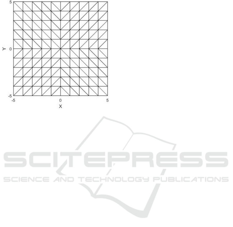
Figure 1: The standard triangulation T
std
in R
2
on [−5,5]
2
.
Remark 2.6. Important for computing CPA Lya-
punov functions is not the shape-matrix itself but the
quantity kX
−1
S
k
p
, where usually p = 2, but for some
applications p = 1 or p = ∞ are more appropriate.
Because all norms on the finite-dimensional vector
space R
n×n
are equivalent there is no fundamental
difference between these norms. It is tempting to as-
sume that the quantity kX
−1
S
k
p
could be related to
the determinant of X
S
, because (n!)
−1
|det X
S
| is well
known to be the volume of the simplex and does not
depend on the choice of x
0
or the order of the dif-
ferences x
i
−x
0
in the shape-matrix. However, as
e.g. shown in (Golub and van Loan, 2013, §2.6.3),
there is no correlation between kX
−1
S
k
p
and |det X
S
|.
Let us give a short discussion on det X
S
, because
we will need it later.
Remark 2.7. That |det X
S
| does not depend on the
choice of x
0
or the order of the differences x
i
−
x
0
in the shape-matrix follows from a volume ar-
gument, but can also be seen algebraically. Let
x
a
i
= (1,x
T
i
)
T
∈ R
n+1
be the vectors x
i
∈ R
n
aug-
mented with 1 in the first position. Define X
a
=

x
a
0
x
a
1
···x
a
n

T
∈ R
(n+1)×(n+1)
. Defining A = (a
i j
) ∈
R
(n+1)×(n+1)
through
a
ii
= 1 for i = 1,. ..,n + 1,
a
i1
= −1 for i = 2, ...,n + 1, and
a
i j
= 0 otherwise,
gives
AX
a
= (x
a
0
,x
a
1
−x
a
0
,. ..,x
a
n
−x
a
0
)
T
=





1 x
T
0
0 (x
1
−x
0
)
T
.
.
.
.
.
.
0 (x
n
−x
0
)
T





.
Laplace expansion on the first row of A and the first
column of AX
a
gives
detA = 1 and det(AX
a
) = 1 ·det X
S
,
i.e. det X
a
= det X
S
. Choosing a different base vector
x
0
and rearranging the order of the differences x
i
−
x
0
corresponds to choosing a permutation matrix P ∈
R
(n+1)×(n+1)
, cf. the discussion after Definition 4.2,
and considering the matrix APX
a
. Since
|det APX
a
| = |det X
a
| = |det X
S
|
the proposition follows.
3 CONSTRUCTION OF CPA
LYAPUNOV FUNCTIONS
Let us explain in detail why the quantity kX
−1
S
k
p
is
of so much interest in our application of computing
CPA Lyapunov functions. To prove that the algo-
rithm in (Giesl and Hafstein, 2014) always succeeds
in computing a CPA Lyapunov functions for any sys-
tem
˙
x = f(x), f ∈ C
2
(R
n
,R
n
), with an exponentially
stable equilibrium at the origin, one uses the fact that
there exists a C
2
Lyapunov function W for the sys-
tem. This function W is used to prove that the linear
programming problem in the algorithm has a feasible
solution for a suitable triangulation.
In the proof in (Giesl and Hafstein, 2014) W is
approximated on S = co(x
0
,x
1
,. ..,x
n
) by its interpo-
lation W
CPA
on S: With
x =
n
∑
i=0
λ
x
i
x
i
∈ S
as the unique convex combination of the vertices, we
set
W
CPA
(x) =
n
∑
i=0
λ
x
i
W (x
i
).
While this obviously approximates the values of W
well on a simplex S with a small diameter h :=
diam(S), e.g. using
|
W (x)−W
CPA
(x)
|
≤
n
∑
i=0
λ
x
i
|
W (x)−W
CPA
(x
i
)
|
≤ h ·max
z∈S
k∇W(z)k
2
,
ICINCO 2021 - 18th International Conference on Informatics in Control, Automation and Robotics
552

this is not sufficient for the proof, because we addi-
tionally need ∇W
CPA
to closely approximate ∇W at
the vertices x
i
, cf. the proof of Theorem 5 in (Giesl
and Hafstein, 2014).
It is not difficult to show that ∇W
CPA
is the con-
stant vector X
−1
S
w, where
w =




W (x
1
) −W (x
0
)
W (x
2
) −W (x
0
)
.
.
.
W (x
n
) −W (x
0
)




,
for all x ∈ S
◦
, cf. Remark 9 in (Giesl and Hafstein,
2014). From this one obtains by Taylor expansion,
cf. (19) in (Giesl and Hafstein, 2014),
[w −X
S
∇W(x
0
)]
i
= (x
i
−x
0
)
T
H
W
(z
i
)(x
i
−x
0
) (3)
for i = 1, 2,..., n, where H
W
is the Hessian matrix of
W and the z
i
are points in S.
Now
k∇W
CPA
−∇W(x
i
)k
p
≤ kX
−1
S
w −∇W (x
0
)k
p
+ k∇W(x
0
) −∇W (x
i
)k
p
and the term k∇W (x
0
) −∇W (x
i
)k
p
is small if the di-
ameter h of the simplex S is small because W ∈ C
2
.
The term kX
−1
S
w −∇W (x
0
)k
p
, however, is not neces-
sarily small even though the diameter h of the simplex
S is small. But we have
kX
−1
S
w −∇W (x
0
)k
p
≤ kX
−1
S
k
p
kw −X
S
∇W(x
0
)k
p
,
and the ith entry of the vector w −X
S
∇W(x
0
) can be
bounded using (3),
|[w −X
S
∇W(x
0
)]
i
| = |(x
i
−x
0
)
T
H
W
(z
i
)(x
i
−x
0
)|
≤ h
2
·sup
z∈S
kH
W
(z)k
2
.
Because of this, the proof in (Giesl and Hafstein,
2014) that the CPA method always succeeds in com-
puting a Lyapunov function if one exists, uses a se-
quence of finite triangulations T
k
where the simplices
become smaller, i.e. h → 0 as k → ∞, but also such
that h
2
·kX
−1
S
k
p
→0 as k → ∞, or, as a sufficient con-
dition, that h ·kX
−1
S
k
p
≤ d is bounded.
Now note that when we scale down the sim-
plex S, i.e. multiply the vertices of S with a number
0 < s < 1, then diam(sS) = s diam(S) and kX
−1
sS
k
p
=
s
−1
kX
−1
S
k
p
. This leads to the following strategy of
obtaining a suitable sequence of triangulations T
k
for
proving that the algorithm in (Giesl and Hafstein,
2014) succeeds in computing a Lyapunov function on
any compact set C , that is contained in the basin of at-
traction of the equilibrium at the origin. For simplic-
ity we ignore some adaptations that have to be made
close to the equilibrium, but do not change the main
idea of the proof:
We have that diam(T
std
) =
√
n and from Remark
2 in (Hafstein and Valfells, 2017) we know that
sup
S∈T
std
kX
−1
S
k
p
≤ 2 for p = 1,2,∞. Fix a constant
s fulfilling 0 < s < 1 and define
T
k
:= {s
k
S
ν
: (s
k
S
ν
) ∩C
◦
6=
/
0}
for k ∈ N
0
. Then for each k ∈ N
0
, T
k
consists of a
finite number of simplices, we have
diam(T
k
) = s
k
√
n
and
sup
s
k
S∈T
k
diam(s
k
S)kX
−1
s
k
S
k
p
≤ s
k
√
n ·s
−k
2 = 2
√
n.
Thus
diam(T
k
) → 0
as k →∞ and
sup
s
k
S∈T
k
diam(s
k
S)kX
−1
s
k
S
k
p
≤ 2
√
n =: d
is bounded. Hence, it follows that W
CPA
and ∇W
CPA
approximate W and ∇W arbitrarily close on C for suf-
ficiently large k.
With identical argumentation an arbitrary se-
quence of triangulations T
k
such that
• diam(T
k
) → 0 for k → 0 and
• there is a bound d such that
sup
S∈T
k
diam(S)kX
−1
S
k
p
≤ d holds for all
k ∈N
0
can be used in the proof in (Giesl and Hafstein, 2014).
The situation explained above led to the def-
inition of the degeneracy of a triangulation and
(h,d)-bounded triangulations in (Giesl and Hafstein,
2015a).
Definition 3.1. We define the degeneracy of the tri-
angulation T to be the quantity
sup
S∈T
diam(S)kX
−1
S
k
2
,
where X
S
is the shape-matrix of S. We say that the tri-
angulation T is (h, d)-bounded for constants h,d >
0, if diam(T ) < h and the degeneracy of T is bounded
by d, i.e. sup
S∈T
diam(S)kX
−1
S
k
2
≤ d.
4 MAIN RESULTS
As explained in the last section, the algorithm seeks
to find a sequence of triangulations T
k
such that each
triangulation T
k
is (h
k
,d)-bounded, where h
k
→ 0 as
k →∞ and d > 0 is a constant independent of k.
Our first main result is Proposition 4.1, which
shows that the concept of (h,d)-bounded triangula-
tions can equivalently be formulated in terms of the
norm and the condition number of the shape-matrices
of the triangulation.
Uniformly Regular Triangulations for Parameterizing Lyapunov Functions
553

Proposition 4.1. Let S = co(x
0
,x
1
,. ..,x
n
) be a sim-
plex and X
S
be its corresponding shape-matrix. Then
1
n
kX
S
k
2
≤ diam(S) ≤ 2
√
nkX
S
k
2
and
1
n
κ
2
(X
S
) ≤ diam(S)kX
−1
S
k
2
≤ 2
√
nκ
2
(X
S
).
Proof. Fix i, j ∈ {0, 1,..., n} such that diam(S) =
kx
i
−x
j
k
2
and k ∈ {1, 2,..., n} such that kX
S
k
∞
=
kx
k
−x
0
k
1
. Then we have
kX
S
k
∞
= kx
k
−x
0
k
1
≤
√
nkx
k
−x
0
k
2
≤
√
nkx
i
−x
j
k
2
=
√
n diam(S)
and
diam(S) = kx
i
−x
j
k
2
≤ kx
i
−x
0
k
2
+ kx
j
−x
0
k
2
≤ kx
i
−x
0
k
1
+ kx
j
−x
0
k
1
≤ 2kX
S
k
∞
.
Hence,
kX
S
k
2
≤
√
nkX
S
k
∞
≤ n diam(S)
≤ 2nkX
S
k
∞
≤ 2n
√
nkX
S
k
2
and
κ
2
(X
S
) = kX
S
k
2
kX
−1
S
k
2
≤ n diam(S)kX
−1
S
k
2
≤ 2n
√
nκ
2
(X
S
).
Thus, a triangulation T is (h, d)-bounded for
some constants h, d > 0, if and only if there exists
constants h
∗
,d
∗
> 0 such that
kX
S
k
2
≤ h
∗
and κ
2
(X
S
) ≤ d
∗
for all S ∈T ,
where X
S
is the shape-matrix corresponding to the
simplex S ∈ T . In either case we define it to be uni-
formly regular:
Definition 4.2 (Uniformly regular triangulations). A
triangulation T in R
n
consisting of simplices with or-
dered vertices is said to be uniformly regular if there
exist constants h,d > 0 such that
diam(S) ≤ h and diam(S)kX
−1
S
k
2
≤ d
for all S ∈ T , or equivalently if there exist constants
h
∗
,d
∗
> 0 such that
kX
S
k
2
≤ h
∗
and κ
2
(X
S
) ≤ d
∗
for all S ∈ T . Here X
S
denotes the shape-matrix of
the simplex S.
We will now prepare our second main result,
showing that a uniformly regular triangulation does
not depend on the order of the vertices in Proposition
4.4. Given a permutation α ∈ Sym(n) of the numbers
{1,2, ...,n}, the permutation matrix P
α
∈R
n×n
is de-
fined through
P
α
e
k
= e
α(k)
for k = 1, 2,. ..,n.
It is not difficult to see that P
−1
α
= P
T
α
and kP
α
k
p
=
kP
−1
α
k
p
= 1 for p ∈ {1,2,∞}. Note that left-
multiplication by P
α
permutes the rows- and right-
multiplication permutes the columns of a vector
or a matrix, e.g. with x = (x
1
,x
2
,. ..,x
n
)
T
and
x
α
=

x
α(1)
,x
α(2)
,. ..,x
α(n)

T
we have P
α
x = x
α
and
x
T
P
α
= x
T
α
.
We have the following simple result.
Lemma 4.3. Let X, P,Q ∈ R
n×n
be matrices, P,Q
nonsingular, and k·k any sub-multiplicative matrix
norm. If
kQk = kQ
−1
k = kPk = kP
−1
k = 1,
then
kQXPk = kXk.
In particular,
kP
α
XP
β
k
p
= kXk
p
for p ∈{1,2,∞}
and for any permutation matrices P
α
,P
β
∈ R
n×n
.
Proof. The first statement follows immediately from
kXk = kQ
−1
QXPP
−1
k ≤ kQ
−1
kkQXPkkP
−1
k
= kQXPk ≤ kQkkXkkPk = kX k.
The second statement follows immediately from the
comments above the lemma.
In the next proposition we show one of our main
results, namely that if a triangulation in R
n
, n ≥ 2,
is (h,d)-bounded for some particular ordering of the
vertices of the simplices, then it is (h,d
∗
)-bounded
for any ordering with d
∗
= d(1 + d
√
n −1). The case
n = 1 is trivial with d
∗
= d.
Proposition 4.4. Let T = {coC
ν
}
ν∈I
be an (h,d)-
bounded triangulation in R
n
, n ≥ 2, and let T
∗
=
{coC
∗
ν
}
ν∈I
be a triangulation consisting of the same
simplices as T , but with a (possibly) different order-
ing of the vertices. Then T
∗
is (h,d
∗
)-bounded, where
d
∗
= d

1 + d
√
n −1

.
Proof. Let S = co(x
0
,x
1
,. ..,x
n
) ∈ T , with shape-
matrix X
S
= (x
1
−x
0
,x
2
−x
0
,. ..,x
n
−x
0
)
T
. Then
S = co(x
β(0)
,x
β(1)
,. ..,x
β(n)
) is also a simplex in T
∗
,
where β is a permutation of {0,1,.. ., n}. If β(0) = 0,
then the shape-matrix X
∗
S
of S in T
∗
has the same
ICINCO 2021 - 18th International Conference on Informatics in Control, Automation and Robotics
554

rows as the shape-matrix X
S
of S in T , just in a (pos-
sibly) different order. Then it follows immediately by
Lemma 4.3 that k(X
∗
S
)
−1
k
2
= kX
−1
S
k
2
and then
diam(S)k(X
∗
S
)
−1
k
2
≤ d ≤ d(1 + d
√
n −1) =: d
∗
.
If β(0) 6= 0, then there is an i ∈ {1,2,.. .,n} such that
β(i) = 0. Define α ∈ Sym
n
through α(i) = β(0) and
α(k) = β(k) for k 6= i and denote by P
α
the permu-
tation matrix defined through P
α
e
k
= e
α(k)
. Then we
have
X
∗
S
= R
i
P
α
X
S
| {z }
=:A
+u(x
0
−x
α(i)
)
T
| {z }
=:v
T
, (4)
where
R
i
:= I −2e
i
e
T
i
and u :=
n
∑
k=1
k6=i
e
k
.
To show (4) we first calculate the left-hand side to be
X
∗
S
=



















x
β(1)
−x
β(0)

T
.
.
.

x
β(i−1)
−x
β(0)

T

x
β(i)
−x
β(0)

T

x
β(i+1)
−x
β(0)

T
.
.
.

x
β(n)
−x
β(0)

T


















=



















x
α(1)
−x
α(i)

T
.
.
.

x
α(i−1)
−x
α(i)

T

x
0
−x
α(i)

T

x
α(i+1)
−x
α(i)

T
.
.
.

x
α(n)
−x
α(i)

T


















.
For the right-hand side of (4) we have
A = R
i
P
α



(x
1
−x
0
)
T
.
.
.
(x
n
−x
0
)
T



= R
i





x
α(1)
−x
0

T
.
.
.

x
α(n)
−x
0

T




=



















x
α(1)
−x
0

T
.
.
.

x
α(i−1)
−x
0

T
−

x
α(i)
−x
0

T

x
α(i+1)
−x
0

T
.
.
.

x
α(n)
−x
0

T


















and
uv
T
=


















x
0
−x
α(i)

T
.
.
.

x
0
−x
α(i)

T
0
T

x
0
−x
α(i)

T
.
.
.

x
0
−x
α(i)

T

















This shows (4). Now
|det A| = |det(R
i
P
α
X
S
)| = |det R
i
|·|det P
α
|·|det X
S
|
= 1 ·1 ·|detX
S
| = |det X
S
|
and by Remark 2.7 we have |det X
S
| = |det X
∗
S
| 6= 0.
Note that 1 + v
T
A
−1
u 6= 0. Indeed, otherwise we
have
0 = u(1 + v
T
A
−1
u)
= (A + uv
T
)A
−1
u
= X
∗
S
A
−1
u,
which is a contradiction because X
∗
S
and A
−1
are in-
vertible and u 6= 0.
Thus we obtain by Lemma 1.1 that


1 + v
T
A
−1
u


=




det(A + uv
T
)
detA




=
|det X
∗
S
|
|det X
S
|
= 1.
Uniformly Regular Triangulations for Parameterizing Lyapunov Functions
555

Further, again by Lemma 1.1, we obtain that


(X
∗
S
)
−1


2
=




A
−1
−
A
−1
uv
T
A
−1
1 + v
T
A
−1
u




2
≤ kA
−1
k
2

1 + kA
−1
k
2
kuv
T
k
2

.
It is easy to see that
kuv
T
k
2
= max
kxk
2
=1
kuv
T
xk
2
≤ max
kxk
2
=1
|v
T
x|kuk
2
≤ kvk
2
√
n −1
= kx
0
−x
α(i)
k
2
√
n −1
≤ diam(S)
√
n −1,
and by Lemma 4.3 we have kA
−1
k
2
=
kX
−1
S
P
−1
α
R
−1
i
k
2
= kX
−1
S
k
2
, from which


(X
∗
S
)
−1


2
≤ kX
−1
S
k
2

1 + kX
−1
S
k
2
diam(S)
√
n −1

≤ kX
−1
S
k
2

1 + d
√
n −1

and then
diam(S)


(X
∗
S
)
−1


2
≤ d

1 + d
√
n −1

=: d
∗
follows.
Since the simplex S ∈ T
∗
was arbitrary, we have
shown that T
∗
is (h,d
∗
)-bounded.
The following proposition is a direct consequence
of Proposition 4.4.
Proposition 4.5. Assume T
k
, k ∈ N
0
, is a sequence of
triangulations in R
n
, such that T
k
is (h
k
,d
k
)-bounded,
and h
k
→ 0 as k → ∞ and d
k
≤ d for all k ∈ N
0
. Let
T
∗
k
, k ∈N
0
, be a sequence of triangulations such that
T
∗
k
consists of the simplices of T
k
, but with a (pos-
sibly) different ordering of the vertices of the sim-
plices. Then there are constants d
∗
k
,d
∗
such that T
∗
k
is
(h
k
,d
∗
k
)-bounded, k ∈N
0
, and d
∗
k
≤ d
∗
for all k ∈N
0
.
Proof. The case n = 1 is trivial and the case n ≥ 2
is obvious from Proposition 4.4 with d
∗
k
= d
k
(1 +
d
k
√
n −1) and d
∗
= d
∗
(1 + d
∗
√
n −1).
We have shown that one can talk about an (h,d)-
bounded triangulation T = {coC
ν
}
ν∈I
, where C
ν
=
{x
0
,x
1
,. ..,x
n
} for every ν ∈ I. That is, the vertices
C
ν
do not have to be ordered n-tuples and can be
sets. The understanding is then that no matter how
the vertices of the simplices are ordered, the resulting
triangulation in R
n
is (h,d)-bounded in the sense of
Definition 3.1. Similarly, if T = {coC
ν
}
ν∈I
, where
C
ν
= (x
0
,x
1
,. ..,x
n
) is an ordered n-tuple for every
ν ∈ I, we can be sure that the corresponding triangu-
lation, where the C
ν
s are changed into sets, is (h,d
∗
)-
bounded in this new sense with d
∗
= d(1 + d
√
n −1).
Thus, one can define for triangulations, of which
the vertices of the simplices are not necessarily or-
dered
Definition 4.6 (Uniformly regular triangulations). A
triangulation T in R
n
consisting of simplices S
ν
=
coC
ν
, C
ν
:= {x
0
,x
1
,··· ,x
n
} is said to be uniformly
regular if there exist constants h,d > 0 such that for
any ordering of the vertices C
ν
of the simplices S
ν
∈T
we have
diam(S) ≤ h and diam(S)kX
−1
S
k
2
≤ d
for all S ∈ T , or equivalently if there exist constants
h
∗
,d
∗
> 0 such that
kX
S
k
2
≤ h
∗
and κ
2
(X
S
) ≤ d
∗
for all S ∈ T . Here X
S
denotes the shape-matrix of
the simplex S with respect to the ordering chosen.
5 CONCLUSIONS
Sequences of triangulations of R
n
having uniform
upper bounds on the diameters and degeneracy of
the simplices are important for the CPA algorithm
to compute continuous and piecewise affine (CPA)
Lyapunov functions for nonlinear systems (Hafstein,
2004; Hafstein, 2005; Giesl and Hafstein, 2014).
In this paper we have eliminated the dependence
of the degeneracy on the ordering of the vertices of
the simplices in the triangulation. Thus, the degen-
eracy can be defined for the simplices as geometrical
objects. Further, we have provided a characterization
of the degeneracy in terms of the condition number of
the shape-matrices.
ACKNOWLEDGEMENT
The research done for this paper was partially sup-
ported by the Icelandic Research Fund (Rann
´
ıs) grant
number 163074-052, Complete Lyapunov functions:
Efficient numerical computation, which is gratefully
acknowledged.
REFERENCES
Albertsson, S., Giesl, P., Gudmundsson, S., and Hafstein,
S. (2020). Simplicial complex with approximate ro-
tational symmetry: A general class of simplicial com-
plexes. J. Comput. Appl. Math., 363:413–425.
ICINCO 2021 - 18th International Conference on Informatics in Control, Automation and Robotics
556

Anderson, J. and Papachristodoulou, A. (2015). Advances
in computational Lyapunov analysis using sum-of-
squares programming. Discrete Contin. Dyn. Syst. Ser.
B, 20(8):2361–2381.
Chesi, G. (2011). Domain of Attraction: Analysis and Con-
trol via SOS Programming. Lecture Notes in Control
and Information Sciences, vol. 415, Springer.
Giesl, P. (2007). Construction of Global Lyapunov Func-
tions Using Radial Basis Functions. Lecture Notes in
Math. 1904, Springer.
Giesl, P. and Hafstein, S. (2014). Revised CPA method to
compute Lyapunov functions for nonlinear systems. J.
Math. Anal. Appl., 410:292–306.
Giesl, P. and Hafstein, S. (2015a). Computation and verifi-
cation of Lyapunov functions. SIAM Journal on Ap-
plied Dynamical Systems, 14(4):1663–1698.
Giesl, P. and Hafstein, S. (2015b). Review of computa-
tional methods for Lyapunov functions. Discrete Con-
tin. Dyn. Syst. Ser. B, 20(8):2291–2331.
Golub, G. and van Loan, C. (2013). Matrix Computations.
John Hopkins University Press, 4 edition.
Hafstein, S. (2004). A constructive converse Lyapunov the-
orem on exponential stability. Discrete Contin. Dyn.
Syst. Ser. A, 10(3):657–678.
Hafstein, S. (2005). A constructive converse Lyapunov
theorem on asymptotic stability for nonlinear au-
tonomous ordinary differential equations. Dynamical
Systems: An International Journal, 20(3):281–299.
Hafstein, S. and Valfells, A. (2017). Study of dynamical
systems by fast numerical computation of Lyapunov
functions. In Proceedings of the 14th International
Conference on Dynamical Systems: Theory and Ap-
plications (DSTA), volume Mathematical and Numer-
ical Aspects of Dynamical System Analysis, pages
220–240.
Hahn, W. (1967). Stability of Motion. Springer, Berlin.
Julian, P., Guivant, J., and Desages, A. (1999). A
parametrization of piecewise linear Lyapunov func-
tions via linear programming. Int. J. Control, 72(7-
8):702–715.
Kamyar, R. and Peet, M. (2015). Polynomial optimization
with applications to stability analysis and control – an
alternative to sum of squares. Discrete Contin. Dyn.
Syst. Ser. B, 20(8):2383–2417.
Khalil, H. (2002). Nonlinear systems. Pearson, 3. edition.
Marin
´
osson, S. (2002). Lyapunov function construction for
ordinary differential equations with linear program-
ming. Dynamical Systems: An International Journal,
17:137–150.
Parrilo, P. (2000). Structured Semidefinite Programs and
Semialgebraic Geometry Methods in Robustness and
Optimiza. PhD thesis: California Institute of Technol-
ogy Pasadena, California.
Ratschan, S. and She, Z. (2010). Providing a basin of attrac-
tion to a target region of polynomial systems by com-
putation of Lyapunov-like functions. SIAM J. Control
Optim., 48(7):4377–4394.
Sastry, S. (1999). Nonlinear Systems: Analysis, Stability,
and Control. Springer.
Sherman, J. and Morrison, W. (1950). Adjustment of an in-
verse matrix corresponding to a change in one element
of a given matrix. Ann. Math. Statist., 21(1):124–127.
Valmorbida, G. and Anderson, J. (2017). Region of attrac-
tion estimation using invariant sets and rational Lya-
punov functions. Automatica, 75:37–45.
Vannelli, A. and Vidyasagar, M. (1985). Maximal Lya-
punov functions and domains of attraction for au-
tonomous nonlinear systems. Automatica, 21(1):69–
80.
Vidyasagar, M. (2002). Nonlinear System Analysis. Clas-
sics in applied mathematics. SIAM, 2. edition.
Yoshizawa, T. (1966). Stability theory by Liapunov’s sec-
ond method. Publications of the Mathematical Society
of Japan, No. 9. The Mathematical Society of Japan,
Tokyo.
Zubov, V. I. (1964). Methods of A. M. Lyapunov and their
application. Translation prepared under the auspices
of the United States Atomic Energy Commission;
edited by Leo F. Boron. P. Noordhoff Ltd, Groningen.
Uniformly Regular Triangulations for Parameterizing Lyapunov Functions
557