Model Predictive Control: A Survey of Dynamic Energy Management

Nsilulu T. Mbungu

1,2,3 a

, Raj M. Naidoo

1 b

, Ramesh C. Bansal

2 c

and Mukwanga W. Siti

3 d

Department of Electrical, Electronic and Computer Engineering, University of Pretoria, Pretoria, South Africa

Department of Electrical and Computer Engineering, University of Sharjah, Sharjah, U.A.E.

Department of Electrical Engineering, Tshwane University of Technology, Pretoria, South Africa

Keywords:

Energy Efﬁciency, Model Predictive Control, Optimal Control, Power System, Demand Response.

Abstract:

This paper presents the structure of the model predictive control (MPC), its development and application

through optimal energy system. The MPC is one of the algorithms that are used in a computer controlled

environment to predict the future behaviour of an explicit process model. It is devised by computing and

adjusting the next sequence of the input variables at each control interval. The MPC is an algorithm in which

the challenge is to optimize the behaviour of a future plant. The optimization sequence starts by sending the

ﬁrst input into the plant and then at each subsequent control interval the entire computation is repeated to reach

the performance index function to follow. MPC offers a variety of applications in a wide range of industries.

This is due to its robustness in the optimal control design of a process. MPC is also widely used in aerospace,

automotive, chemical and food processing applications. This study describes the implementation of the energy

management scheme through the use of MPC design.

1 INTRODUCTION

Managing the energy system has transformed the con-

ﬁguration of a conventional power grid in terms of

coordinating the optimal power ﬂow, minimising the

system power losses and voltage stability on the elec-

trical network (Abdi et al., 2017a; Siti et al., 2019;

Abdi et al., 2017b; Mbungu et al., 2019a; Adefarati

et al., 2019; Foley et al., 2020). Currently, several re-

search works try to look for the alternative approaches

of dealing with different grid’s challenges, which con-

sists of analysing the system protection of the electri-

cal system and optimal integration and coordination

of energy mix system. The objective of these ap-

proaches aims to improve the efﬁciency of the power

system, which must be based on dynamic modelling

strategy.

MPC is frequently used in the industry as an op-

timal control strategy due to its ability to handle hard

system constraints. MPC system design offers the

possibility of controlling the input system and the out-

put constraints (Mesbah, 2016; Mbungu et al., 2018;

Kale and Chipperﬁeld, 2005) as well as the incremen-

https://orcid.org/0000-0003-0498-5065

https://orcid.org/0000-0002-2439-4505

https://orcid.org/0000-0002-1725-2648

https://orcid.org/0000-0002-8085-4967

tal constraints of the control signal (Mbungu et al.,

2020). Manufacturing process has been widely in-

ﬂuenced by developing the implementation of MPC

due to its approach to resolve and manage the uncer-

tainty of a processing system. It predicts the future

behaviour and keeps the input and output signal in the

acceptable optimal operation level.

Through the MPC strategy, a controller of a given

system can handle multiple inputs, multiple outputs

plant model that are subject to diverse constraints.

The MPC algorithm is also valued for its robustness in

handling unexpected process and system behaviour.

Therefore, this research works contributes on imple-

mentation strategy of a system behavior based on

MPC design. The approach aims to analyse the dy-

namic performance of the energy management under

the smart grid environment.

2 SYSTEM MODELLING

2.1 State-space Model

Consider a given function f (x, u) with its internal sys-

tem, in which the vector space is known as the state-

space. If this structure is also lumped together and

has ﬁnite state-space, then, the state-space equations

Mbungu, N., Naidoo, R., Bansal, R. and Siti, M.

Model Predictive Control: A Survey of Dynamic Energy Management.

DOI: 10.5220/0010522201230129

In Proceedings of the 18th International Conference on Informatics in Control, Automation and Robotics (ICINCO 2021), pages 123-129

ISBN: 978-989-758-522-7

123

can describe the system. It is essential to note that

modelling of this type of structure in a state-space

model must satisfy the three superposition of the state

and the output equations and the linearity propri-

ety of state-space (Holkar and Waghmare, 2010; Se-

borg et al., 2010; Bishop, 2007; Lee, 2009; Mayne

et al., 2000; Dahleh et al., 2004; Rossiter, 2003; Ma-

ciejowski, 2002; Rawlings and Mayne, 2009). The

state of the system is the basis of the state-space rep-

resentation. It also considers the value of updating

internal elements of the system. This procedure can

change independently from the system output. The

function f (x, u) in the state-space model is constituted

of three components, namely input variables (u) or

manipulated variables (MVs), output variables (y) or

controlled variables (CVs), and the state variables (x)

(Mbungu et al., 2016; Mbungu et al., 2017b; Wang,

2009; Holkar and Waghmare, 2010; Seborg et al.,

2010; Bishop, 2007; Lee, 2009; Mayne et al., 2000;

Dahleh et al., 2004; Rossiter, 2003; Maciejowski,

2002; Rawlings and Mayne, 2009). The vectors be-

low describe these components as:

u(t) =













, y(t) =













, x(t) =













(1)

where m the number of input into the system, q the

number of output of the plant mode, and n the number

of state that deﬁnes the system or order of state-space.

2.1.1 Continuous-time System

If the function f (x, u, t) is considered as the state

evolution equation of a given system, and the out-

put vector y(t) can be described by the function of

the state variable and MVs over a given time t as

g(x, u, t), which is the instantaneous output equation

(Dahleh et al., 2004; Rossiter, 2003; Maciejowski,

2002; Rawlings and Mayne, 2009). Therefore, the re-

lation below can describe the system in a continuous

time model as:

˙x(t) = f (x(t), u(t), t) (2a)

y(t) = g(x(t), u(t), t) (2b)

where t ∈ R or R

, and ˙x(t) is the rate of change

of the state variables. Equation 2 can be simpliﬁed

in compact linear and time-invariant relations, which

describe the continuous state space model of a given

system as:

˙x(t) = Ax(t)+ Bu(t) (3a)

y(t) = Cx(t) + Du(t) (3b)

where A, B,C, and D are respectively, the state ma-

trix of dimension, input matrix, output matrix, and

feed forward matrix. For t ≥ 0, x(t) ∈ R

, u(t) ∈

, and y ∈ R

these involve that dim[A] = n × n,

dim[B] = n × m, dim[C] = q × n, and dim[D] = q × m.

Due to the absence of direct feed through on the sys-

tem model developed in (Mbungu et al., 2016; Wang,

2009; Mbungu et al., 2017b), it is assumed that the

feed forward matrix is zero.

2.1.2 Discrete-time System

The discrete-time system model is considered a stan-

dard state-space model. Nowadays, all modern ap-

plications in control systems are discretised or dig-

italised for more accurate evaluation and robustness

of the design. The discrete time system offers the

possibility of determining the output of the system

in real time by using past information of the input.

The technical approach should be followed regard-

ing the amount of input information which deﬁnes

the present output. From Eq. 3a, the discrete time

system in a state-space model is developed. This con-

sists of using Euler’s forward approximation method

(Mbungu et al., 2016; Mbungu et al., 2017b; Dahleh

et al., 2004). Suppose that the system is operated at a

given period T , the discretization of state evolution in

that time for (x, u, t) can be determined as (Mbungu

et al., 2016; Mbungu et al., 2017b; Dahleh et al.,

2004; Rossiter, 2003; Maciejowski, 2002; Rawlings

and Mayne, 2009).

x((t + 1)T ) − x(tT )

= Ax(tT ) + Bu(tT ) (4)

If it is supposed that the parameters (tT ) can be

replaced by (k), where k ∈ Z denotes the time sample,

Eq. 4 can therefore be rewritten as follows

x(k + 1) = (I + TA)x(k) + T Bu(k) = A

x(k) + B

u(k)

(5)

By combining Eq. 5 with the output function of

continuous state space model Eq. 3b which is sup-

posed to be discretised by Euler’s forward approxi-

mation like Eq. 43a, the linear discrete state space

model can be described as

x(k + 1) = A

x(k) + T B

u(k) (6a)

y(k) = C

x(k) + D

u(k) (6b)

where A

is the discrete state matrix, B

is discrete

input matrix, C

is discrete output matrix, and D

is the discrete feedforward matrix. It is also impor-

tant to notice that all discrete time matrices of Eq. 6

have the same dimension with the continuous matri-

ces that are deﬁned in Eq 3. However, in most cases,

ICINCO 2021 - 18th International Conference on Informatics in Control, Automation and Robotics

124

for example, in predictive control, it can sometimes

be assumed that the feed-forward matrix D

equals

to zero (Mbungu et al., 2016; Mbungu et al., 2017b;

Zhang et al., 2014; Wang, 2009; Rossiter, 2003; Ma-

ciejowski, 2002; Rawlings and Mayne, 2009; Ma

et al., 2011; Xie et al., 2007). This is dependent on the

system design due to the principle of receding horizon

(Wang, 2009). In this study, the linear discrete state

space model is used to design the system.

2.2 Augmented State Space Model

Suppose that at a given MV with sample k, ﬁnding the

relationship between the sample k and the instant be-

fore it, i.e., k − 1, this relation could describe the aug-

mented state space model. Equation 6a could, there-

fore, be rewritten as (Mbungu et al., 2017b; Wang,

2009)

x(k +1)−x (k) = A

(x(k) −x(k −1))+B

(u(k) −u(1−1))

(7)

Through Eq. 7, the increment of state variables

and the MV can be rewritten respectively by ∆x(k +

1) = x(k + 1) − x(k), ∆x(k) = x(k) − x(k − 1) and

∆u(k) = u(k) − u(k − 1). By considering these in-

cremental function and Eq. 7, the increment of the

state-space equation is therefore expressed as

∆x(k + 1) = A

∆x(k) + B

∆u(k) (8)

As the system input is changed to the increment

of MV, it is, therefore, a question of connecting the

increment of state vector to the CV. This method in-

troduces a new state vector of the system that is de-

veloped as follows.

(k) =



∆x(k)

∆y(k)



(9)

where x

denotes the augmented state vector.

From Eqs. 8 and 9, the output vector at the sample

(k + 1) needs to be determined for the stability of the

system. If, at a given sample k of a CV, the designed

model can predict a future CV at the sample (k + 1).

By using the developed strategy of Eq. 7, which can

be identiﬁed with the effect of CV in Eq. 9, thus, Eq.

6a as a function of current and future CV with D

= 0

is expressed as follows.

y(k + 1) − y(k) = C

(x(k + 1) − x(k)) = C

∆x(k + 1)

(10)

By substituting Eq. 8 in Eq. 10, the relation-

ship between the current and predicted CV can be ex-

pressed as follows.

y(k + 1) − y(k) = C

∆x(k) +C

∆u(k) (11)

Equations 12a and 12b deﬁne the compact format

of the augmented state-space model, which derives

from Eqs. 8, 9, and 11 as follows.

(k + 1) = A

(k) + B

∆u(k) (12a)

y(k) = C

(12b)

where A





, B





, C





(k + 1) =



∆x

y(k)



, and 0



0 0 ... 0



with 0

as a zero column vector of n dimension. The aug-

mented state space system is also used in MPC design

(Wang, 2009).

3 PREDICTIVE CONTROL

The MPC approach is the composition of three base

components of the predictive controller. These are

the prediction, optimisation and receding horizon im-

plementation. The advantages of predictive control

strategy are its stability of driver for constrained sys-

tems. Moreover, due to the opportunity of real-time

computation and the improvement of the predictive

controller efﬁciency, the application predictive con-

trol has extended many controller structures that in-

clude high-speed sampling systems (Cannon, 2015).

3.1 Prediction

By considering the dynamic model of discrete-time

linear state-space model Eq. 6a and the MPC sam-

ple time strategy, to generate the predicted behaviour

of a given plant system consists of assuming that at

sampling instant kth, the future state vector is in a re-

lationship with the next input. This strategy is exe-

cuted for N sampling intervals. If only at each given

predicted MV sequence when the model is simulated

forward over a given prediction horizon, the corre-

sponding sequence of predicted state is, therefore,

generated to describe the future sequence behaviour

of the system. The vector state and below input deﬁne

the predicted sequence of the discrete-time dynamic

model.

x(k) =







x(k + 1|K)

x(k + 2|K)

x(k + 3|K)

x(k + N|K)







, u(k) =







u(k|K)

u(k + 1|K)

u(k + 2|K)

x(k + N − 1|K)







(13)

where x(k + i|K) and u(k + i|K) are respectively the

state vector and MV at a time (k + i) and the parame-

ter k of each variable denotes the predicted sampling

Model Predictive Control: A Survey of Dynamic Energy Management

125

instant. Through Eq. 13, the demonic model of linear

discrete state-space is rewritten in predictive environ-

ment as:

x(k + i + 1|k) = A

x(k + 1|k) + B

u(k + 1|k) (14)

with i = 0, 1, ..., N, and for the initial condition i.e.

i = 0 the state vector is x(k|k) = x(k ).

3.2 Optimisation

References (Wang, 2009; Holkar and Waghmare,

2010; Seborg et al., 2010) describe the predicted con-

trol law computation framework. The optimisation

strategy of MPC is based on minimising anticipated

performance cost. The predicted sequence of state

and MV play an inﬂuential role in the optimisation

strategy. Equation 15 deﬁnes the optimal approach to

predictive control as:

J(K) =

∑

i=0

(k + i|k)Qx(k + i|k) + u

(k + i|k)Ru(k + i|k)]

(15)

where J(k) denotes the performance index of pre-

dicted sequences, and Q and R are the positive def-

inite weighting matrices. But Q or R can also be a

positive semi-deﬁnite matrix. It is also important to

notice that Q and R are diagonal matrices that con-

tain only the positive elements. It has been noted that

the performance index is a function of state and MV

at each instant k. During the optimization strategy of

predicted input sequence which consists of minimiz-

ing Eq. 15 to ﬁnd the minimum argument of the input

sequence, at each instant the optimal MV can be cal-

culated as:

∗

(k) = argmin

J(k) (16)

It is also important to note that ﬁnding the mini-

mum MV can be subject to the input, state, and output

constraints. Therefore, these can be included in the

optimization strategy to determine the optimal solu-

tion. The structure of the restrictions in MPC design

will be established further in section 4.

3.3 Receding Horizon Implementations

Once the initial value is computed, i.e. at i = 0 by

using Eqs. 13 and 16 under a ﬁnite horizon, the op-

timal predicted MV sequence that is introduced into

the plant through the MPC control law is determined

as follows.

u(k) = u

∗

(k|k) (17)

For k = 0, 1, ..., N, at each sampling instant as de-

scribed in (Wang, 2009; Holkar and Waghmare, 2010;

Seborg et al., 2010) the same process that is computed

for the ﬁrst element is then repeated at each sampling

instant. The effect of repeating the optimisation of

future time instants describes the online optimisation

strategy of predictive control. This strategy deﬁnes

the receding horizon approach that keeps the predic-

tion horizon at the same length. The concept of feed-

back as described in (Holkar and Waghmare, 2010;

Seborg et al., 2010) determines the degree of robust-

ness of the system.

4 MPC DESIGN

If the dynamic of state-space design for a given dig-

ital mode Eq. 12 can verify either the controllability

or the observable laws, this dynamic model can also

be implanted in MPC controller. The MPC design

entails controlling the optimum approach that the ob-

servation sets at each predicted sequence as deﬁned in

Eq. 15, which is deﬁned as a quadratic equation. This

performance index can develop in terms of MPC gain

for the robustness of the designed controller (Wang,

2009). Thus, the performance index can be rewritten

in function of CVs and the targets of the system as

follows (Mbungu et al., 2016; Mbungu et al., 2017b;

Wang, 2009).

J(k) = (Y (k) − r

)

(Y (k) − r

R(k)) (18)

where J(k), R(k) and r

are the output system,

target to follow, turning parameter respectively. Af-

ter computation of a given sample k with a given

predicted horizon N

and a given control horizon N

through an MPC design, the optimum output of sys-

tem is descried in (Mbungu et al., 2018; Tungadio

et al., 2018; Mbungu et al., 2017a).

Afterwards, optimising the given system by us-

ing the MPC design is the effect of implanting a

quadratic equation as described in (Mbungu et al.,

2016; Mbungu et al., 2017b; Wang, 2009), whuch

can compute whether a constraining or unconstrain-

ing plant model. This consists of ﬁnding the argu-

ment of CV in relation with the minimum value of the

objective function of the MPC gain.

4.1 Quadratic Programming

A quadratic programming offers several advantages in

the industrial environment due to its opportunity of a

real-time application. This consists of safely writing a

jacket software implementation and the possibility to

update and change the code (Holkar and Waghmare,

2010; Seborg et al., 2010; Mbungu et al., 2020). If

the objective function of a given plant model in MPC

ICINCO 2021 - 18th International Conference on Informatics in Control, Automation and Robotics

126

computation is subject to some linear inequality con-

straints, ﬁnding the optimum control solution of the

MVs in receding horizon implementation consists of

resolving a quadratic programming equation below

J(k) = H(k)u(k) +

u(k)

G(k)u(k) (19a)

Mu(k) ≤ γ (19b)

where M and γ are constraints matrix and vector. Eq.

19b can be either or not combined with the equal-

ity constraints (Seborg et al., 2010). This system re-

striction mostly depends on what the controller has to

achieve on the performance of a given model.

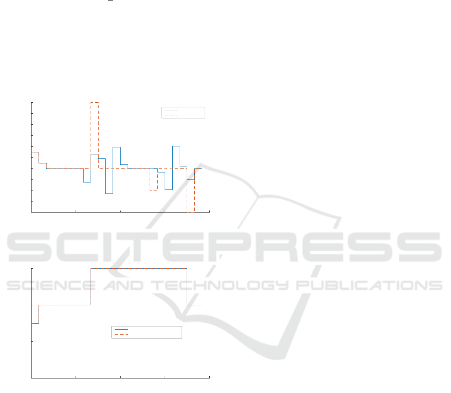
time (h)

0 6 12 18 24

Energy (kWh)

-40

-30

-20

-10

Optimum ∆e

target ∆e

Figure 1: Daily TOU-MPC cost of electricity vs target of

electricity cost.

time(h)

0 6 12 18 24

Energy(kWh)

Optimal Energy Demand

Reference Energy Demand

Figure 2: Daily Prepaid-MPC cost of electricity vs target of

electricity cost.

5 IMPLEMENTATION ANALYSIS

This section consists of analysing the dynamic behav-

ior of MPC design. The simulation of the results are

based on the data developed in (Mbungu et al., 2016;

Holkar and Waghmare, 2010) of the energy manage-

ment system for a commercial load demand. Besides,

this research study deals on the possibility of ﬁnding

the dynamic energy system of the increment of the

control variable. The strategy implements the demand

response scheme based the energy management in the

consumers side (Mbungu et al., 2019b), namely real-

time electricity pricing.

5.1 Simulation Analysis

Table 1 provides different biased values that are used

to simulate the dynamic behavior of the given data.

The system implementation computed different time

of use (TOU) and prepaid electricity tariff as de-

scribed in Table 1. The simulation of the results is

presented in Figs. 1 and 2. Figure 1 gives the dy-

namic behavior of the optimal energy that ﬂows on

the system. It is necessary to notice that this model

computes only the increment of the control signal as

described by the canonic form of state space model

in Eqs. 12a and 12b. Besides, the performance in-

dex of the MPC design as described in Eq. 18, with

its developed strategy which includes constraints and

simpliﬁed model of the objective function (Eqs. 19a

and 19b) are computed in the fashion of the increment

model. It is also important to notice that Fig. 2 is not

computed by the augmented model.

5.2 Discussion Analysis

Tables 2 and 3 present different values of the energy

cost and the saving energy. When it is about to com-

pare the results of the optimal input signal with target

input as described in Figs. 1 and 2, it is clearly shown

that this result is roughly running close to one another

for the increment signal during TOU computation,

and both signals (target and optimal energy demand)

are close in prepaid mode. However, at some time,

the optimal result does not follow the target energy.

This interpretation can be controversial in the context

of energy-saving and optimal computation. Neverthe-

less, the total cost of energy and the percentage of

the energy cost saving as described in Table 2 gives

another proﬁle of the system performance. Besides,

Table 3 and Fig. 2 present perfect results which are

not often guaranteed during the computation process.

Based on this approach of interpreting the simulations

results, it can be seen that the system dynamics of the

proposed MPC scheme provides satisfactory results

to the consumer side. This is due to the important

value of the optimal energy cost and the signiﬁcant

percentage rate of the cost-saving.

6 CONCLUSION

The MPC is an optimisation strategy because it of-

fers the opportunity of computing the control vari-

Model Predictive Control: A Survey of Dynamic Energy Management

127

Table 1: Turning parameter and Energy tariffs.

Tariff scheme Weighted coefﬁcient Energy prices (R/kWh)

Off-peak (TOU) 1 0.6150

Standard (TOU) 1 and 5 1.073

Peak(TOU) 1.0526 and 1.143 4.115

Prepaid 2 1.2774

Table 2: TOU Cost of energy and percent of costs analysis.

Type of strategy Cost (Rand) Parameters Saving analysis (%)

Cost to pay 2254.3 Cost-target 48.1818

Target cost 1086.2 MPC cost 38.1196

Optimal cost 895.3235 Cost-saving 61.8804

Table 3: Prepaid Cost of energy and percent of costs analysis.

Type of strategy Cost (Rand) Parameters Saving analysis (%)

Cost to pay 1475.4 Cost-target 52.3810

Target cost 772.8270 MPC cost 52.3810

Optimal cost 772.8270 Cost-saving 47.6190

ables based on a given target. This optimal con-

trol method aimed to minimising the cost of electric-

ity for a given electrical system. It was found that

the model is robust in conjunction with consumers

actions. It involves creation of an optimal strategy

where the user can custom the amount of electricity

to use. The optimisation tactics of the MVs for an

MPC is an online algorithm that can compute any lin-

ear model in the real-time environment. The MPC ap-

proach is also considered as a suitable strategy algo-

rithm to be implemented in smart grid technology due

to its robustness in the optimal control solution. The

MPC can also perform a control problem as an opti-

misation problem that is made by an on-line optimi-

sation with receding horizon implementation. Thus,

the real-time optimisation through the quadratic pro-

gramming strategy in the framework of the MPC per-

forms a suitable scheme between data transfer and op-

timisation calculation. It also aims to resolve at each

sampling time the optimal controller within the given

set-point. Besides, the system provides satisfactory

performance in terms of energy-saving and cost opti-

misation. Therefore, future research work can look at

different implementation strategy of the MPC design

through a dynamic energy metering based on sensors

networking within the applications of the smart tech-

nologies.

REFERENCES

Abdi, H., Beigvand, S. D., and La Scala, M. (2017a). A

review of optimal power ﬂow studies applied to smart

grids and microgrids. Renewable and Sustainable En-

ergy Reviews, 71:742–766.

Abdi, H., Beigvand, S. D., and La Scala, M. (2017b). A

review of optimal power ﬂow studies applied to smart

grids and microgrids. Renewable and Sustainable En-

ergy Reviews, 71:742–766.

Adefarati, T., Bansal, R. C., Naidoo, R. M., and Mbungu,

N. T. (Aug 12-15, 2019). Techno-economic evalua-

tion of a grid connected microgrid-cogeneration sys-

tem using wind turbines, microturbine and battery sys-

tem. In International Conference on Applied Energy,

aster

as, Sweden.

Bishop, R. H. (2007). Mechatronic systems, sensors, and

actuators: fundamentals and modeling. CRC press,

Texas, USA, 2nd ed edition.

Cannon, M. (2015). C21 Model Predictive Control. Uni-

versity of Oxford, Oxford, Tech. Rep.

Dahleh, M., Dahleh, M. A., and Verghese, G. (2004).

Lectures on dynamic systems and control. A+ A,

4(100):1–100.

Foley, A. M., McIlwaine, N., Morrow, D. J., Hayes, B. P.,

Zehir, M. A., Mehigan, L., Papari, B., Edrington,

C. S., Baran, M., et al. (2020). A critical evaluation

of grid stability and codes, energy storage and smart

loads in power systems with wind generation. Energy,

205:117671.

Holkar, K. and Waghmare, L. (2010). An overview of

model predictive control. International Journal of

Control and Automation, 3(4):47–63.

ICINCO 2021 - 18th International Conference on Informatics in Control, Automation and Robotics

128

Kale, M. and Chipperﬁeld, A. (2005). Stabilized mpc

formulations for robust reconﬁgurable ﬂight control.

Control Engineering Practice, 13(6):771–788.

Lee, J. H. (2009). A Lecture on Model Predictive Control.

Pan American Advanced Studies Institute Program on

Process Systems Engineering.

Ma, J., Qin, S. J., Li, B., and Salsbury, T. (2011). Economic

model predictive control for building energy systems.

IEEE, Anaheim, USA.

Maciejowski, J. M. (2002). Predictive control: with con-

straints. Pearson education, London, UK.

Mayne, D. Q., Rawlings, J. B., Rao, C. V., and Scokaert,

P. O. (2000). Constrained model predictive control:

Stability and optimality. Automatica, 36(6):789–814.

Mbungu, N. T., Bansal, R. C., and Naidoo, R. (2019a).

Smart energy coordination of autonomous residential

home. IET Smart Grid, 2(3):336–346.

Mbungu, N. T., Bansal, R. C., Naidoo, R., Miranda, V., and

Bipath, M. (2018). An optimal energy management

system for a commercial building with renewable en-

ergy generation under real-time electricity prices. Sus-

tainable Cities and Society, 41:392–404.

Mbungu, N. T., Bansal, R. C., Naidoo, R. M., Bettayeb, M.,

Siti, M. W., and Bipath, M. (2020). A dynamic energy

management system using smart metering. Applied

Energy, 280:115990.

Mbungu, N. T., Naidoo, R., Bansal, R. C., and Bipath,

M. (2017a). Optimisation of grid connected hybrid

photovoltaic–wind–battery system using model pre-

dictive control design. IET Renewable Power Gen-

eration, 11(14):1760–1768.

Mbungu, N. T., Naidoo, R. M., and Bansal, R. C. (2017b).

Real-time electricity pricing: TOU-MPC based en-

ergy management for commercial buildings. Energy

Procedia, 105:3419–3424.

Mbungu, N. T., Naidoo, R. M., Bansal, R. C., and Vahid-

inasab, V. (2019b). Overview of the optimal smart

energy coordination for microgrid applications. IEEE

Access, 7:163063–163084.

Mbungu, T., Naidoo, R., Bansal, R., and Bipath, M. (2016).

Smart SISO-MPC based energy management system

for commercial buildings: Technology trends. In Fu-

ture Technologies Conference (FTC), pages 750–753,

San Francisco, USA.

Mesbah, A. (2016). Stochastic model predictive control: An

overview and perspectives for future research. IEEE

Control Systems Magazine, 36(6):30–44.

Rawlings, J. B. and Mayne, D. Q. (2009). Model predictive

control: Theory and design. Nob Hill Pub, New York,

USA.

Rossiter, J. A. (2003). Model-based predictive control: a

practical approach. CRC press, New York, USA.

Seborg, D. E., Mellichamp, D. A., Edgar, T. F., and

Doyle III, F. J. (2010). Process dynamics and control.

John Wiley & Sons, USA, 3rd ed edition.

Siti, M. W., Tungadio, D. H., Sun, Y., Mbungu, N. T., and

Tiako, R. (2019). Optimal frequency deviations con-

trol in microgrid interconnected systems. IET Renew-

able Power Generation, 13(13):2376–2382.

Tungadio, D. H., Bansal, R. C., Siti, M. W., and Mbungu,

N. T. (2018). Predictive active power control of

two interconnected microgrids. Technology and

Economics of Smart Grids and Sustainable Energy,

3(3):1–15.

Wang, L. (2009). Model predictive control system design

and implementation using MATLAB

. Springer Sci-

ence & Business Media, Girona, Spain.

Xie, L., Li, P., and Wozny, G. (2007). Chance constrained

nonlinear model predictive control. Assessment and

Future Directions of Nonlinear Model Predictive Con-

trol, pages 295–304.

Zhang, Y., Liu, B., Zhang, T., and Guo, B. (2014). An intel-

ligent control strategy of battery energy storage sys-

tem for microgrid energy management under forecast

uncertainties. International Journal of Electrochemi-

cal Science, 9(8):4190–4204.

Model Predictive Control: A Survey of Dynamic Energy Management

129